Understanding Effect Size from Differences in Mean
Synopsis
Working Definition : Working from a sample of a population and trying to estimate something about the world
We are trying to generalize from what we measure about the world from a sample.
Statistical Inference
Estimate Effect Size
Quantify precision of the result[ Confidence Interval / standard error]
Doing Hypothesis testing: [What is chance that the difference is zero? Or in another words, it happened by chance?]
Imports
import numpy as np
import scipy as sp
import scipy.stats as stats
import matplotlib as plt
import matplotlib.pyplot as plt
from ipywidgets import interact, interactive, fixed
import ipywidgets as widgets
from
# seed the random number generator so we all get the same results
np.random.seed(17)

# some nice colors from http://colorbrewer2.org/
COLOR1 = '#7fc97f'
COLOR2 = '#beaed4'
COLOR3 = '#fdc086'
COLOR4 = '#ffff99'
COLOR5 = '#386cb0'
%matplotlib inline
Part 1
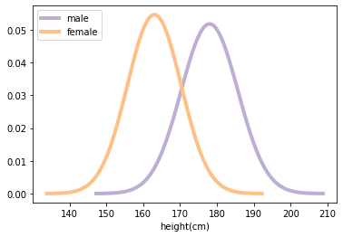
Population distribution
mu1, sig1 = 178, 7.7
male_height = stats.norm(mu1, sig1); male_height
<scipy.stats._distn_infrastructure.rv_frozen at 0x7f18e0daac70>
mu2, sig2 = 163, 7.3
female_height = stats.norm(mu2, sig2); female_height
<scipy.stats._distn_infrastructure.rv_frozen at 0x7f1819eb5730>
Function to evaluate normal(Gaussian) PDF
def eval_pdf(rv, n=4):
    mean, std = rv.mean(), rv.std()
    xs = np.linspace(mean - n*std, mean + n*std, 100)
    ys = rv.pdf(xs)
    return xs, ys
xs_male, ys_male = eval_pdf(male_height)
xs_female, ys_female = eval_pdf(female_height)
fig= plt.figure()
ax = fig.gca()
ax.plot(xs_male, ys_male, label='male', linewidth=4, color=COLOR2)
ax.plot(xs_female, ys_female, label='female', linewidth=4, color=COLOR3)
plt.xlabel('height(cm)')
plt.legend(loc='upper left')
plt.show()

Random Sampling from distribution/population
male_sample = male_height.rvs(1000); male_sample.shape
(1000,)
female_sample = female_height.rvs(1000); female_sample.shape
(1000,)
Mean of sample will be close to population but not exactly same
mean1, std1 = male_sample.mean(), male_sample.std()
mean1, std1
(178.16511665818112, 7.84199617128995)
mean2, std2 = female_sample.mean(), female_sample.std()
mean2, std2
(163.48610226651135, 7.382384919896662)
difference_in_mean = mean1-mean2
difference_in_mean
14.679014391669767
relative_difference_by_sample = (2*difference_in_mean/(mean1+mean2))*100
relative_difference_by_sample
8.59298230392402
relative_difference_by_distribution = (2*difference_in_mean/(mu1+mu2))*100
relative_difference_by_distribution
8.609392605084908
relative_difference_by_male = difference_in_mean/mu1*100
relative_difference_by_male
8.24663729869088
relative_difference_by_female = difference_in_mean/mu2*100
relative_difference_by_female
9.005530301637894
Which one is correct?
Here things are symmetric so you can express in either way
What about taking avg?
There may be situation where you have a treatment group and control group. There you might want to do
\(Diff_{treatment}/ mean_{control}\)
Part 2
Understanding the overlap, threshold, misclassification rate
Alternative way to quantify difference is to see how much they overlap
Simple threshold
simple_thresh = (mean1 + mean2)/2; simple_thresh
170.82560946234622
Threshold(more appropriate)
thresh = (mean1*std2+mean2*std1)/(std1+std2); thresh
170.6040359174722
Overlap
How many male below threshold ?
male_below_thresh = sum(male_sample<thresh); male_below_thresh
164
How many female above threshold ?
female_above_thresh = sum(female_sample>thresh); female_above_thresh
174
The “overlap” is the area under the curves that ends up on the wrong side of the threshold
male_overlap = male_below_thresh / len(male_sample)
female_overlap = female_above_thresh / len(female_sample)
male_overlap, female_overlap

# overlap = (male_overlap + female_overlap)
(0.164, 0.174)
Misclassification Rate
misclassification_rate = (male_overlap+female_overlap)/2; misclassification_rate
0.16899999999999998
Probability of superiority
Another way to quantify the difference between distributions is what’s called “probability of superiority”, which is a problematic term.
In this context it’s the probability that a randomly-chosen man is taller than a randomly-chosen woman.
sum(male_sample > female_sample), (male_sample> female_sample).mean()
(918, 0.918)
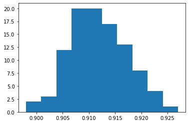
Distribution of Superiority
male_sample[:5]
array([178.44105417, 170.49028233, 170.94885314, 188.07981499,
       171.51692076])
np.random.shuffle(male_sample)
male_sample[:5]
array([180.02059072, 185.18602683, 177.45366243, 176.95014285,
       186.13226315])
s = []
for i in range(100):
    np.random.shuffle(male_sample)
    np.random.shuffle(female_sample)
    s.append((male_sample> female_sample).mean())
prob_sup_sample = np.array(s)
plt.hist(prob_sup_sample)
plt.show()

@interact
def plot_prob_sup(n_trials=(100, 1000), n_bins=(20, 40)):
    s = []
    for i in range(n_trials):
        np.random.shuffle(male_sample)
        np.random.shuffle(female_sample)
        s.append((male_sample> female_sample).mean())
    prob_sup_sample = np.array(s)
    mean = np.mean(prob_sup_sample)
    std = np.std(prob_sup_sample)
    plt.title(f"$\mu$ {mean:0.01f} \n $\sigma$ {std:0.03f} \n n {n_trials}")

    plt.hist(prob_sup_sample, bins=n_bins, color=COLOR1)
    plt.axvline(x=mean, color=COLOR3)
    plt.axvline(x=mean-2*std, color=COLOR2)
    plt.axvline(x=mean+2*std, color=COLOR2)
    plt.xlim(.890, .950)
    plt.xlabel("N[male_height > female_height]")
    plt.show()
Note
Overlap(or misclassification rate) & “probability of superiority” have 2 good properties:
As probabilities, they don’t depend on UOM- Comparable between studies
Expressed in Operational terms ( sense of what practical effect the difference makes)
Cohens’ Effect Size
Difference in mean , standardized by dividing by std. dev
\(d = \frac{\bar{x_1} - \bar{x_2}}{s}\)
Pooled standard deviation
\(s = \sqrt{\frac{n_1{s_1}^2+n_2{s_2}^2}{n_1+n_2}}\)
Implementation cohen’s effectsize
def cohen_effectsize(grp1, grp2):
    diff = grp1.mean() - grp2.mean()

    n1, n2 = len(grp1), len(grp2)
    var1 = grp1.var()
    var2 = grp2.var()

    pooled_var = (n1*var1+n2*var2)/(n1+n2)

    d = diff/np.sqrt(pooled_var)
    return d
cohen_effectsize(male_sample, female_sample)
1.9274780043619493
Implementation overlap_superiority
def overlap_superiority(control, treatment, n=1000):

    control_sample = control.rvs(n)
    treatment_sample = treatment.rvs(n)
#     mean1, std1 = control_sample.mean(), control_sample.std()
#     mean2, std2 = treatment_sample.mean(), control_sample.std()
# #     treatment_sample.mean()
#     thresh = (mean1*std2+mean2*std1)/(std1+std2)
    thresh = (control.mean()+treatment.mean())/2

    control_above = sum(control_sample > thresh)
    treatment_below = sum(treatment_sample < thresh)
    overlap = (control_above + treatment_below)/n
    superiority =  (treatment_sample> control_sample).mean()
    return overlap , superiority
overlap_superiority(male_height, female_height)
(1.672, 0.083)
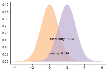
def plot_pdfs(cohen_d=2):
    control = stats.norm(0,1)
    treatment = stats.norm(cohen_d,1)
    xs, ys = eval_pdf(control)
    plt.fill_between(xs, ys, label='control',
                        color=COLOR3, alpha=0.7)
    xs, ys = eval_pdf(treatment)
    plt.fill_between(xs, ys, label='treatment',
                        color=COLOR2, alpha=0.7)
    o, s = overlap_superiority(control, treatment)
    plt.text(0, 0.05, 'overlap ' + str(o))
    plt.text(0, 0.15, 'superiority ' + str(s))
    plt.show()
plot_pdfs(2)

slider = widgets.FloatSlider(min=0, max=4.1, value=2)
interactive(plot_pdfs, cohen_d=slider)
Note
Cohen effect size non dimensional
Can be used to calculate overlap and probability of superiority
