Sampling
Synopsis
Effect on proportion
Percentages
Bad as percentage can have different intuition for different ranges
Difference is subjective
Odds Ratio
LOR
Most appropriate (symmetric)
Choosing Effect Size indicator is driven by context and familiarity. Use something which makes sense to individuals/ audience
Precision
How precise is data?
Sources of Errors
Sampling Errors
Is my sample representative of population?
Measurement Errors
UOM
Improper Recording
Random Errors
Least important
Only one with mathematical model behind it, so it’s used all the time in statistics classes
Imports
import numpy as np
import scipy as sp
import scipy.stats as stats
import matplotlib as mpl
import matplotlib.pyplot as plt
from ipywidgets import interact, interactive, fixed
import ipywidgets as widgets
import pandas as pd
from IPython.display import display, display_html
import bqplot

from bqplot import LinearScale, Hist, Figure, Axis, ColorScale

from bqplot import pyplot as pltbq
# import seaborn as sns
# seed the random number generator so we all get the same results
np.random.seed(17)

# some nice colors from http://colorbrewer2.org/
COLOR1 = '#7fc97f'
COLOR2 = '#beaed4'
COLOR3 = '#fdc086'
COLOR4 = '#ffff99'
COLOR5 = '#386cb0'

mpl.rcParams['figure.figsize'] = (8.0, 9.0)
%matplotlib inline
Part 1
Estimate Avg. weight of man & woman in US
Quantify uncertainity in estimate
Approach =>
Simulate many exp
Compare how results vary from one experiment to another
Start by assuming distribution and move on show how to eliminate this assumption (solve without it)
#Weight of woman(in kg)

weight = stats.lognorm(0.23, 0, 70.8)
weight.mean(), weight.std()
(72.69764573296688, 16.944043048498038)
help(stats.lognorm)
Help on lognorm_gen in module scipy.stats._continuous_distns object:

class lognorm_gen(scipy.stats._distn_infrastructure.rv_continuous)
 |  lognorm_gen(momtype=1, a=None, b=None, xtol=1e-14, badvalue=None, name=None, longname=None, shapes=None, extradoc=None, seed=None)
 |
 |  A lognormal continuous random variable.
 |
 |  %(before_notes)s
 |
 |  Notes
 |  -----
 |  The probability density function for `lognorm` is:
 |
 |  .. math::
 |
 |      f(x, s) = \frac{1}{s x \sqrt{2\pi}}
 |                \exp\left(-\frac{\log^2(x)}{2s^2}\right)
 |
 |  for :math:`x > 0`, :math:`s > 0`.
 |
 |  `lognorm` takes ``s`` as a shape parameter for :math:`s`.
 |
 |  %(after_notes)s
 |
 |  A common parametrization for a lognormal random variable ``Y`` is in
 |  terms of the mean, ``mu``, and standard deviation, ``sigma``, of the
 |  unique normally distributed random variable ``X`` such that exp(X) = Y.
 |  This parametrization corresponds to setting ``s = sigma`` and ``scale =
 |  exp(mu)``.
 |
 |  %(example)s
 |
 |  Method resolution order:
 |      lognorm_gen
 |      scipy.stats._distn_infrastructure.rv_continuous
 |      scipy.stats._distn_infrastructure.rv_generic
 |      builtins.object
 |
 |  Methods defined here:
 |
 |  fit(self, data, *args, **kwds)
 |      Return MLEs for shape (if applicable), location, and scale
 |      parameters from data.
 |
 |      MLE stands for Maximum Likelihood Estimate.  Starting estimates for
 |      the fit are given by input arguments; for any arguments not provided
 |      with starting estimates, ``self._fitstart(data)`` is called to generate
 |      such.
 |
 |      One can hold some parameters fixed to specific values by passing in
 |      keyword arguments ``f0``, ``f1``, ..., ``fn`` (for shape parameters)
 |      and ``floc`` and ``fscale`` (for location and scale parameters,
 |      respectively).
 |
 |      Parameters
 |      ----------
 |      data : array_like
 |          Data to use in calculating the MLEs.
 |      arg1, arg2, arg3,... : floats, optional
 |          Starting value(s) for any shape-characterizing arguments (those not
 |          provided will be determined by a call to ``_fitstart(data)``).
 |          No default value.
 |      kwds : floats, optional
 |          - `loc`: initial guess of the distribution's location parameter.
 |          - `scale`: initial guess of the distribution's scale parameter.
 |
 |          Special keyword arguments are recognized as holding certain
 |          parameters fixed:
 |
 |          - f0...fn : hold respective shape parameters fixed.
 |            Alternatively, shape parameters to fix can be specified by name.
 |            For example, if ``self.shapes == "a, b"``, ``fa`` and ``fix_a``
 |            are equivalent to ``f0``, and ``fb`` and ``fix_b`` are
 |            equivalent to ``f1``.
 |
 |          - floc : hold location parameter fixed to specified value.
 |
 |          - fscale : hold scale parameter fixed to specified value.
 |
 |          - optimizer : The optimizer to use.  The optimizer must take ``func``,
 |            and starting position as the first two arguments,
 |            plus ``args`` (for extra arguments to pass to the
 |            function to be optimized) and ``disp=0`` to suppress
 |            output as keyword arguments.
 |
 |      Returns
 |      -------
 |      mle_tuple : tuple of floats
 |          MLEs for any shape parameters (if applicable), followed by those
 |          for location and scale. For most random variables, shape statistics
 |          will be returned, but there are exceptions (e.g. ``norm``).
 |
 |      Notes
 |      -----
 |      This fit is computed by maximizing a log-likelihood function, with
 |      penalty applied for samples outside of range of the distribution. The
 |      returned answer is not guaranteed to be the globally optimal MLE, it
 |      may only be locally optimal, or the optimization may fail altogether.
 |      If the data contain any of np.nan, np.inf, or -np.inf, the fit routine
 |      will throw a RuntimeError.
 |
 |      When the location parameter is fixed by using the `floc` argument,
 |      this function uses explicit formulas for the maximum likelihood
 |      estimation of the log-normal shape and scale parameters, so the
 |      `optimizer`, `loc` and `scale` keyword arguments are ignored.
 |
 |      Examples
 |      --------
 |
 |      Generate some data to fit: draw random variates from the `beta`
 |      distribution
 |
 |      >>> from scipy.stats import beta
 |      >>> a, b = 1., 2.
 |      >>> x = beta.rvs(a, b, size=1000)
 |
 |      Now we can fit all four parameters (``a``, ``b``, ``loc`` and ``scale``):
 |
 |      >>> a1, b1, loc1, scale1 = beta.fit(x)
 |
 |      We can also use some prior knowledge about the dataset: let's keep
 |      ``loc`` and ``scale`` fixed:
 |
 |      >>> a1, b1, loc1, scale1 = beta.fit(x, floc=0, fscale=1)
 |      >>> loc1, scale1
 |      (0, 1)
 |
 |      We can also keep shape parameters fixed by using ``f``-keywords. To
 |      keep the zero-th shape parameter ``a`` equal 1, use ``f0=1`` or,
 |      equivalently, ``fa=1``:
 |
 |      >>> a1, b1, loc1, scale1 = beta.fit(x, fa=1, floc=0, fscale=1)
 |      >>> a1
 |      1
 |
 |      Not all distributions return estimates for the shape parameters.
 |      ``norm`` for example just returns estimates for location and scale:
 |
 |      >>> from scipy.stats import norm
 |      >>> x = norm.rvs(a, b, size=1000, random_state=123)
 |      >>> loc1, scale1 = norm.fit(x)
 |      >>> loc1, scale1
 |      (0.92087172783841631, 2.0015750750324668)
 |
 |  ----------------------------------------------------------------------
 |  Methods inherited from scipy.stats._distn_infrastructure.rv_continuous:
 |
 |  __init__(self, momtype=1, a=None, b=None, xtol=1e-14, badvalue=None, name=None, longname=None, shapes=None, extradoc=None, seed=None)
 |      Initialize self.  See help(type(self)) for accurate signature.
 |
 |  cdf(self, x, *args, **kwds)
 |      Cumulative distribution function of the given RV.
 |
 |      Parameters
 |      ----------
 |      x : array_like
 |          quantiles
 |      arg1, arg2, arg3,... : array_like
 |          The shape parameter(s) for the distribution (see docstring of the
 |          instance object for more information)
 |      loc : array_like, optional
 |          location parameter (default=0)
 |      scale : array_like, optional
 |          scale parameter (default=1)
 |
 |      Returns
 |      -------
 |      cdf : ndarray
 |          Cumulative distribution function evaluated at `x`
 |
 |  expect(self, func=None, args=(), loc=0, scale=1, lb=None, ub=None, conditional=False, **kwds)
 |      Calculate expected value of a function with respect to the
 |      distribution by numerical integration.
 |
 |      The expected value of a function ``f(x)`` with respect to a
 |      distribution ``dist`` is defined as::
 |
 |                  ub
 |          E[f(x)] = Integral(f(x) * dist.pdf(x)),
 |                  lb
 |
 |      where ``ub`` and ``lb`` are arguments and ``x`` has the ``dist.pdf(x)``
 |      distribution. If the bounds ``lb`` and ``ub`` correspond to the
 |      support of the distribution, e.g. ``[-inf, inf]`` in the default
 |      case, then the integral is the unrestricted expectation of ``f(x)``.
 |      Also, the function ``f(x)`` may be defined such that ``f(x)`` is ``0``
 |      outside a finite interval in which case the expectation is
 |      calculated within the finite range ``[lb, ub]``.
 |
 |      Parameters
 |      ----------
 |      func : callable, optional
 |          Function for which integral is calculated. Takes only one argument.
 |          The default is the identity mapping f(x) = x.
 |      args : tuple, optional
 |          Shape parameters of the distribution.
 |      loc : float, optional
 |          Location parameter (default=0).
 |      scale : float, optional
 |          Scale parameter (default=1).
 |      lb, ub : scalar, optional
 |          Lower and upper bound for integration. Default is set to the
 |          support of the distribution.
 |      conditional : bool, optional
 |          If True, the integral is corrected by the conditional probability
 |          of the integration interval.  The return value is the expectation
 |          of the function, conditional on being in the given interval.
 |          Default is False.
 |
 |      Additional keyword arguments are passed to the integration routine.
 |
 |      Returns
 |      -------
 |      expect : float
 |          The calculated expected value.
 |
 |      Notes
 |      -----
 |      The integration behavior of this function is inherited from
 |      `scipy.integrate.quad`. Neither this function nor
 |      `scipy.integrate.quad` can verify whether the integral exists or is
 |      finite. For example ``cauchy(0).mean()`` returns ``np.nan`` and
 |      ``cauchy(0).expect()`` returns ``0.0``.
 |
 |      The function is not vectorized.
 |
 |      Examples
 |      --------
 |
 |      To understand the effect of the bounds of integration consider
 |
 |      >>> from scipy.stats import expon
 |      >>> expon(1).expect(lambda x: 1, lb=0.0, ub=2.0)
 |      0.6321205588285578
 |
 |      This is close to
 |
 |      >>> expon(1).cdf(2.0) - expon(1).cdf(0.0)
 |      0.6321205588285577
 |
 |      If ``conditional=True``
 |
 |      >>> expon(1).expect(lambda x: 1, lb=0.0, ub=2.0, conditional=True)
 |      1.0000000000000002
 |
 |      The slight deviation from 1 is due to numerical integration.
 |
 |  fit_loc_scale(self, data, *args)
 |      Estimate loc and scale parameters from data using 1st and 2nd moments.
 |
 |      Parameters
 |      ----------
 |      data : array_like
 |          Data to fit.
 |      arg1, arg2, arg3,... : array_like
 |          The shape parameter(s) for the distribution (see docstring of the
 |          instance object for more information).
 |
 |      Returns
 |      -------
 |      Lhat : float
 |          Estimated location parameter for the data.
 |      Shat : float
 |          Estimated scale parameter for the data.
 |
 |  isf(self, q, *args, **kwds)
 |      Inverse survival function (inverse of `sf`) at q of the given RV.
 |
 |      Parameters
 |      ----------
 |      q : array_like
 |          upper tail probability
 |      arg1, arg2, arg3,... : array_like
 |          The shape parameter(s) for the distribution (see docstring of the
 |          instance object for more information)
 |      loc : array_like, optional
 |          location parameter (default=0)
 |      scale : array_like, optional
 |          scale parameter (default=1)
 |
 |      Returns
 |      -------
 |      x : ndarray or scalar
 |          Quantile corresponding to the upper tail probability q.
 |
 |  logcdf(self, x, *args, **kwds)
 |      Log of the cumulative distribution function at x of the given RV.
 |
 |      Parameters
 |      ----------
 |      x : array_like
 |          quantiles
 |      arg1, arg2, arg3,... : array_like
 |          The shape parameter(s) for the distribution (see docstring of the
 |          instance object for more information)
 |      loc : array_like, optional
 |          location parameter (default=0)
 |      scale : array_like, optional
 |          scale parameter (default=1)
 |
 |      Returns
 |      -------
 |      logcdf : array_like
 |          Log of the cumulative distribution function evaluated at x
 |
 |  logpdf(self, x, *args, **kwds)
 |      Log of the probability density function at x of the given RV.
 |
 |      This uses a more numerically accurate calculation if available.
 |
 |      Parameters
 |      ----------
 |      x : array_like
 |          quantiles
 |      arg1, arg2, arg3,... : array_like
 |          The shape parameter(s) for the distribution (see docstring of the
 |          instance object for more information)
 |      loc : array_like, optional
 |          location parameter (default=0)
 |      scale : array_like, optional
 |          scale parameter (default=1)
 |
 |      Returns
 |      -------
 |      logpdf : array_like
 |          Log of the probability density function evaluated at x
 |
 |  logsf(self, x, *args, **kwds)
 |      Log of the survival function of the given RV.
 |
 |      Returns the log of the "survival function," defined as (1 - `cdf`),
 |      evaluated at `x`.
 |
 |      Parameters
 |      ----------
 |      x : array_like
 |          quantiles
 |      arg1, arg2, arg3,... : array_like
 |          The shape parameter(s) for the distribution (see docstring of the
 |          instance object for more information)
 |      loc : array_like, optional
 |          location parameter (default=0)
 |      scale : array_like, optional
 |          scale parameter (default=1)
 |
 |      Returns
 |      -------
 |      logsf : ndarray
 |          Log of the survival function evaluated at `x`.
 |
 |  nnlf(self, theta, x)
 |      Return negative loglikelihood function.
 |
 |      Notes
 |      -----
 |      This is ``-sum(log pdf(x, theta), axis=0)`` where `theta` are the
 |      parameters (including loc and scale).
 |
 |  pdf(self, x, *args, **kwds)
 |      Probability density function at x of the given RV.
 |
 |      Parameters
 |      ----------
 |      x : array_like
 |          quantiles
 |      arg1, arg2, arg3,... : array_like
 |          The shape parameter(s) for the distribution (see docstring of the
 |          instance object for more information)
 |      loc : array_like, optional
 |          location parameter (default=0)
 |      scale : array_like, optional
 |          scale parameter (default=1)
 |
 |      Returns
 |      -------
 |      pdf : ndarray
 |          Probability density function evaluated at x
 |
 |  ppf(self, q, *args, **kwds)
 |      Percent point function (inverse of `cdf`) at q of the given RV.
 |
 |      Parameters
 |      ----------
 |      q : array_like
 |          lower tail probability
 |      arg1, arg2, arg3,... : array_like
 |          The shape parameter(s) for the distribution (see docstring of the
 |          instance object for more information)
 |      loc : array_like, optional
 |          location parameter (default=0)
 |      scale : array_like, optional
 |          scale parameter (default=1)
 |
 |      Returns
 |      -------
 |      x : array_like
 |          quantile corresponding to the lower tail probability q.
 |
 |  sf(self, x, *args, **kwds)
 |      Survival function (1 - `cdf`) at x of the given RV.
 |
 |      Parameters
 |      ----------
 |      x : array_like
 |          quantiles
 |      arg1, arg2, arg3,... : array_like
 |          The shape parameter(s) for the distribution (see docstring of the
 |          instance object for more information)
 |      loc : array_like, optional
 |          location parameter (default=0)
 |      scale : array_like, optional
 |          scale parameter (default=1)
 |
 |      Returns
 |      -------
 |      sf : array_like
 |          Survival function evaluated at x
 |
 |  ----------------------------------------------------------------------
 |  Methods inherited from scipy.stats._distn_infrastructure.rv_generic:
 |
 |  __call__(self, *args, **kwds)
 |      Freeze the distribution for the given arguments.
 |
 |      Parameters
 |      ----------
 |      arg1, arg2, arg3,... : array_like
 |          The shape parameter(s) for the distribution.  Should include all
 |          the non-optional arguments, may include ``loc`` and ``scale``.
 |
 |      Returns
 |      -------
 |      rv_frozen : rv_frozen instance
 |          The frozen distribution.
 |
 |  __getstate__(self)
 |
 |  __setstate__(self, state)
 |
 |  entropy(self, *args, **kwds)
 |      Differential entropy of the RV.
 |
 |      Parameters
 |      ----------
 |      arg1, arg2, arg3,... : array_like
 |          The shape parameter(s) for the distribution (see docstring of the
 |          instance object for more information).
 |      loc : array_like, optional
 |          Location parameter (default=0).
 |      scale : array_like, optional  (continuous distributions only).
 |          Scale parameter (default=1).
 |
 |      Notes
 |      -----
 |      Entropy is defined base `e`:
 |
 |      >>> drv = rv_discrete(values=((0, 1), (0.5, 0.5)))
 |      >>> np.allclose(drv.entropy(), np.log(2.0))
 |      True
 |
 |  freeze(self, *args, **kwds)
 |      Freeze the distribution for the given arguments.
 |
 |      Parameters
 |      ----------
 |      arg1, arg2, arg3,... : array_like
 |          The shape parameter(s) for the distribution.  Should include all
 |          the non-optional arguments, may include ``loc`` and ``scale``.
 |
 |      Returns
 |      -------
 |      rv_frozen : rv_frozen instance
 |          The frozen distribution.
 |
 |  interval(self, alpha, *args, **kwds)
 |      Confidence interval with equal areas around the median.
 |
 |      Parameters
 |      ----------
 |      alpha : array_like of float
 |          Probability that an rv will be drawn from the returned range.
 |          Each value should be in the range [0, 1].
 |      arg1, arg2, ... : array_like
 |          The shape parameter(s) for the distribution (see docstring of the
 |          instance object for more information).
 |      loc : array_like, optional
 |          location parameter, Default is 0.
 |      scale : array_like, optional
 |          scale parameter, Default is 1.
 |
 |      Returns
 |      -------
 |      a, b : ndarray of float
 |          end-points of range that contain ``100 * alpha %`` of the rv's
 |          possible values.
 |
 |  mean(self, *args, **kwds)
 |      Mean of the distribution.
 |
 |      Parameters
 |      ----------
 |      arg1, arg2, arg3,... : array_like
 |          The shape parameter(s) for the distribution (see docstring of the
 |          instance object for more information)
 |      loc : array_like, optional
 |          location parameter (default=0)
 |      scale : array_like, optional
 |          scale parameter (default=1)
 |
 |      Returns
 |      -------
 |      mean : float
 |          the mean of the distribution
 |
 |  median(self, *args, **kwds)
 |      Median of the distribution.
 |
 |      Parameters
 |      ----------
 |      arg1, arg2, arg3,... : array_like
 |          The shape parameter(s) for the distribution (see docstring of the
 |          instance object for more information)
 |      loc : array_like, optional
 |          Location parameter, Default is 0.
 |      scale : array_like, optional
 |          Scale parameter, Default is 1.
 |
 |      Returns
 |      -------
 |      median : float
 |          The median of the distribution.
 |
 |      See Also
 |      --------
 |      rv_discrete.ppf
 |          Inverse of the CDF
 |
 |  moment(self, n, *args, **kwds)
 |      n-th order non-central moment of distribution.
 |
 |      Parameters
 |      ----------
 |      n : int, n >= 1
 |          Order of moment.
 |      arg1, arg2, arg3,... : float
 |          The shape parameter(s) for the distribution (see docstring of the
 |          instance object for more information).
 |      loc : array_like, optional
 |          location parameter (default=0)
 |      scale : array_like, optional
 |          scale parameter (default=1)
 |
 |  rvs(self, *args, **kwds)
 |      Random variates of given type.
 |
 |      Parameters
 |      ----------
 |      arg1, arg2, arg3,... : array_like
 |          The shape parameter(s) for the distribution (see docstring of the
 |          instance object for more information).
 |      loc : array_like, optional
 |          Location parameter (default=0).
 |      scale : array_like, optional
 |          Scale parameter (default=1).
 |      size : int or tuple of ints, optional
 |          Defining number of random variates (default is 1).
 |      random_state : {None, int, `~np.random.RandomState`, `~np.random.Generator`}, optional
 |          If `seed` is `None` the `~np.random.RandomState` singleton is used.
 |          If `seed` is an int, a new ``RandomState`` instance is used, seeded
 |          with seed.
 |          If `seed` is already a ``RandomState`` or ``Generator`` instance,
 |          then that object is used.
 |          Default is None.
 |
 |      Returns
 |      -------
 |      rvs : ndarray or scalar
 |          Random variates of given `size`.
 |
 |  stats(self, *args, **kwds)
 |      Some statistics of the given RV.
 |
 |      Parameters
 |      ----------
 |      arg1, arg2, arg3,... : array_like
 |          The shape parameter(s) for the distribution (see docstring of the
 |          instance object for more information)
 |      loc : array_like, optional
 |          location parameter (default=0)
 |      scale : array_like, optional (continuous RVs only)
 |          scale parameter (default=1)
 |      moments : str, optional
 |          composed of letters ['mvsk'] defining which moments to compute:
 |          'm' = mean,
 |          'v' = variance,
 |          's' = (Fisher's) skew,
 |          'k' = (Fisher's) kurtosis.
 |          (default is 'mv')
 |
 |      Returns
 |      -------
 |      stats : sequence
 |          of requested moments.
 |
 |  std(self, *args, **kwds)
 |      Standard deviation of the distribution.
 |
 |      Parameters
 |      ----------
 |      arg1, arg2, arg3,... : array_like
 |          The shape parameter(s) for the distribution (see docstring of the
 |          instance object for more information)
 |      loc : array_like, optional
 |          location parameter (default=0)
 |      scale : array_like, optional
 |          scale parameter (default=1)
 |
 |      Returns
 |      -------
 |      std : float
 |          standard deviation of the distribution
 |
 |  support(self, *args, **kwargs)
 |      Return the support of the distribution.
 |
 |      Parameters
 |      ----------
 |      arg1, arg2, ... : array_like
 |          The shape parameter(s) for the distribution (see docstring of the
 |          instance object for more information).
 |      loc : array_like, optional
 |          location parameter, Default is 0.
 |      scale : array_like, optional
 |          scale parameter, Default is 1.
 |      Returns
 |      -------
 |      a, b : float
 |          end-points of the distribution's support.
 |
 |  var(self, *args, **kwds)
 |      Variance of the distribution.
 |
 |      Parameters
 |      ----------
 |      arg1, arg2, arg3,... : array_like
 |          The shape parameter(s) for the distribution (see docstring of the
 |          instance object for more information)
 |      loc : array_like, optional
 |          location parameter (default=0)
 |      scale : array_like, optional
 |          scale parameter (default=1)
 |
 |      Returns
 |      -------
 |      var : float
 |          the variance of the distribution
 |
 |  ----------------------------------------------------------------------
 |  Data descriptors inherited from scipy.stats._distn_infrastructure.rv_generic:
 |
 |  __dict__
 |      dictionary for instance variables (if defined)
 |
 |  __weakref__
 |      list of weak references to the object (if defined)
 |
 |  random_state
 |      Get or set the RandomState object for generating random variates.
 |
 |      This can be either None, int, a RandomState instance, or a
 |      np.random.Generator instance.
 |
 |      If None (or np.random), use the RandomState singleton used by np.random.
 |      If already a RandomState or Generator instance, use it.
 |      If an int, use a new RandomState instance seeded with seed.
Note
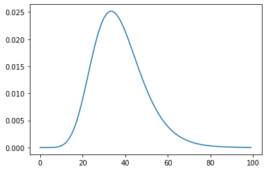
Log normal distribution is specified by 3 parameters
\(\sigma\) - Shape parameter or Standard deviation of Distribution
\(m\) - Scale parameter (median) shrinking or stretching the graphs
\(\theta\) or (\(\mu\)) - Location parameter ; specifying where it is located in map
For log normal distribution. Check following links
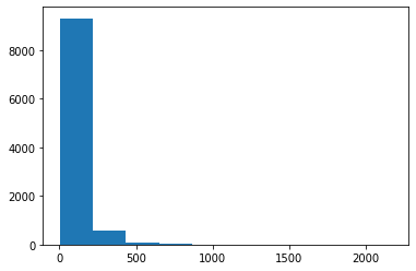
rv = stats.lognorm(1, 0, 50) # Don't know shape , location , median
# xs = np.linspace(1, 100, 100)
ys = rv.rvs(10000)
plt.hist(ys)
(array([9.308e+03, 5.550e+02, 8.500e+01, 3.000e+01, 1.000e+01, 3.000e+00,
        4.000e+00, 3.000e+00, 0.000e+00, 2.000e+00]),
 array([1.12258114e+00, 2.17935158e+02, 4.34747735e+02, 6.51560312e+02,
        8.68372890e+02, 1.08518547e+03, 1.30199804e+03, 1.51881062e+03,
        1.73562320e+03, 1.95243578e+03, 2.16924835e+03]),
 <BarContainer object of 10 artists>)
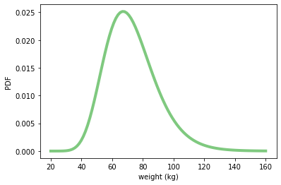
# For women weight
weight = stats.lognorm(0.23, 0, 70.8)
weight.mean(), weight.std()
(72.69764573296688, 16.944043048498038)
xs = np.linspace(20, 160, 100)
ys = weight.pdf(xs)

plt.plot(xs, ys, linewidth=4, color=COLOR1)
plt.xlabel('weight (kg)')
plt.ylabel('PDF')
plt.show()
def make_sample(n=100):
    sample = weight.rvs(n)
    return sample
sample = make_sample(100)
sample.mean(), sample.std()
(73.04819598338332, 16.22111742103728)
def sample_stat(sample):
    return sample.mean()
sample_stat(sample)
73.04819598338332
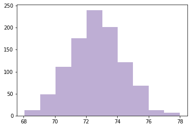
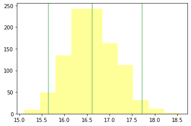
Simulating experiment 1000 times
def computing_sampling_distribution(n=100, iters=1000):
    stats = [sample_stat(make_sample(n)) for i in range(iters)]
    return np.array(stats)
sample_means = computing_sampling_distribution(n=100, iters=1000)
plt.hist(sample_means, color=COLOR2)
plt.show()
@interact
def sim(n=[10,20,50,100, 200, 1000, 10000], iters=[100, 1000, 10000]):
    sample_means = computing_sampling_distribution(n, iters)
    mean = sample_means.mean()
    std = sample_means.std()
    plt.hist(sample_means, bins=30, color=COLOR2)
    plt.axvline(mean, color=COLOR4)
    plt.axvline(mean -3*std, color=COLOR5)
    plt.axvline(mean +3*std, color=COLOR5)

    conf_int = np.percentile(sample_means, [2.5, 97.5]) # 95% confidence interval
    plt.axvline(conf_int[0], color=COLOR1)
    plt.axvline(conf_int[1], color=COLOR1)
    plt.ylabel("count")
    plt.xlabel(f"sample_means(n = {n})")
    plt.title(f" iters={iters},  $\mu_s$={mean:0.4f},  $\sigma_s$={std:0.4f}")
    plt.show()
Application for Sim Monitor
caption = widgets.Label(value='The values of slider1 and slider2 are synchronized')
sliders1, slider2 = widgets.IntSlider(description='Slider 1'),\
                    widgets.IntSlider(description='Slider 2')
l = widgets.link((sliders1, 'value'), (slider2, 'value'))
display(caption, sliders1, slider2)
Simple plot Linked to output widget
%matplotlib widget
widget_plot = widgets.Output()
with widget_plot:
    widget_plot.clear_output()
    ax.clear()
    fig, ax = plt.subplots(1,1)
#     display(ax.figure)
    plt.show()
widget_plot
ax.plot(range(1, 100))
fig.canvas.draw()
---------------------------------------------------------------------------
NameError                                 Traceback (most recent call last)
<ipython-input-21-203552d8af35> in <module>
----> 1 ax.plot(range(1, 100))
      2 fig.canvas.draw()

NameError: name 'ax' is not defined
ax.clear()
ax.plot(range(1, 20))
fig.canvas.draw()
# @interact
# def update_plot(n=2):
#     ax.clear()
#     ax.plot(np.linspace(1,100,100)**n)
#     fig.canvas.draw()
widget_plot
widget_pow = widgets.IntSlider(value=2,min=0, max=5)
widget_pow
def update_plot(n=2):
    ax.clear()
    ax.plot(np.linspace(1,100,100)**n)
    fig.canvas.draw()

def handle_change(change):
    update_plot(change.new)
widget_pow.observe(handle_change, "value")
---------------------------------------------------------------------------
NameError                                 Traceback (most recent call last)
<ipython-input-23-cc35b1b6381a> in <module>
----> 1 widget_pow.observe(handle_change, "value")

NameError: name 'widget_pow' is not defined
widgets.VBox([widget_plot, widget_pow])
---------------------------------------------------------------------------
NameError                                 Traceback (most recent call last)
<ipython-input-24-cb580b1392d7> in <module>
----> 1 widgets.VBox([widget_plot, widget_pow])

NameError: name 'widget_pow' is not defined
Lognorm Application
widgets.SelectionSlider(
    options=[1,2, 5, 6, 10],
    value=1,
    description='n',
    disabled=False,
    continuous_update=False,
    orientation='horizontal',
    readout=True
)
def sample_stat(sample, kind='mean'):
    if kind =='mean':
        return sample.mean()
    elif kind == 'coeff_variation':
        return sample.mean()/sample.std()
    elif kind == 'min':
        return sample.min()
    elif kind == 'max':
        return sample.max()
    elif kind == 'median':
        return np.percentile(sample, 50)
    elif kind == 'p10':
        return np.percentile(sample, 10)
    elif kind == 'p90':
        return np.percentile(sample, 90)
    elif kind == 'IQR':
        return np.percentile(sample, 75) - np.percentile(sample, 25)

def make_sample(rv, n=100):
    sample = rv.rvs(n)
    return sample

def computing_sampling_distribution(rv, n=100, iters=1000, kind='mean'):
    stats = [sample_stat(make_sample(rv, n), kind) for i in range(iters)]
    return np.array(stats)
sample_stat(sample, kind='mean')
fig, axes = plt.subplots(nrows=2, ncols=2)
axes
ax0, ax1, ax2, ax3 = axes.flatten()
# def figure(figsize=None):
#     'Temporary workaround for traditional figure behaviour with the ipympl widget backend'
#     fig = plt.figure()
#     if figsize:
#         w, h =  figsize
#     else:
#         w, h = plt.rcParams['figure.figsize']
#     fig.canvas.layout.height = str(h) + 'in'
#     fig.canvas.layout.width = str(w) + 'in'
#     return fig


def update_text(ax, x, y, s, align='right'):
    ax.text(x, y, s,
            horizontalalignment=align,
            verticalalignment='top',
            transform=ax.transAxes)

# class KindRange(object):
#     def __init__(self, kind, min_d, max_d):
#         self.kind = kind
#         self.min_d = min_d
#         self.max_d = max_d

class LogNormVisualizer(object):

    def __init__(self, shape, loc, median, xs=np.linspace(20, 160, 100)):
        plt.close('all')
        self.shape = shape
        self.loc = loc
        self.median = median
        self.w_shape = widgets.FloatText(value=shape, description='shape',disabled=False)
        self.w_loc = widgets.FloatText(value=loc, description='loc',disabled=False)
        self.w_median = widgets.FloatText(value=median, description='median',disabled=False)
        self.w_n = widgets.SelectionSlider(
                                options=[10,20,50,100, 200, 1000, 10000],
                                value=10,
                                description='n',
                                disabled=False,
                                continuous_update=False,
                                orientation='horizontal',
                                readout=True
                            )

        self.w_kind = widgets.Dropdown(
                                    options=['mean', 'coeff_variation', 'min', 'max', 'median', 'p10', 'p90', 'IQR'],
                                    value='mean',
                                    description='Statisitics',
                                    disabled=False,
                                    continuous_update=False,
                                    orientation='horizontal',
                                    readout=True
                                )
        self.kind = self.w_kind.value
        self.w_iters = widgets.SelectionSlider(
                                options=[100,500, 1000, 5000, 10000],
                                value=100,
                                description='iters',
                                disabled=False,
                                continuous_update=False,
                                orientation='horizontal',
                                readout=True
                            )
        self.rv = stats.lognorm(shape, loc, median)
        self.w_rv = widgets.Output()
        plt.close()
        with self.w_rv:
            self.w_rv.clear_output()
            self.fig, axes = plt.subplots(nrows=4, ncols=1)
            self.ax1, self.ax2, self.ax3, self.ax4 = axes
            self.ax1.set_title("Log Normal Distribution")
            self.ax2.set_title("Statistics")
            self.ax3.set_title("Stat_Variation_n")
            self.ax3.set_title("Stat_Variation_iter")
            self.fig.canvas.toolbar_visible = False
            self.fig.canvas.header_visible = False
            self.fig.canvas.footer_visible = False
#             self.fig.canvas.layout.width = '100%'
#             self.fig.canvas.layout.height = '6in'
#             self.fig.canvas.layout.width = '6in'
            self.fig.canvas.resizable = True
            self.fig.canvas.capture_scroll = True
            self.fig.tight_layout()

        self.range_store = {}
        self.w_range_min = widgets.FloatText(value=0, description='r_min',disabled=False)
        self.w_range_max = widgets.FloatText(value=100, description='r_max',disabled=False)
        self.w_range_reinit = widgets.Button(disabled=False, description='ReInitialize')
        self.w_rv.layout.display = 'flex-grow'
        self.xs = xs
        self.sample_d = None
        self.r_min = None
        self.r_max = None
        self.df = pd.DataFrame(columns=['n', 'iters', 'kind','mean_d','std_d'])
        self.update_rv()
        self.link_widgets()

#         self.update_rv_plot()
#         self.update_stat_plot()

    def init_kind_range_store(self, kind, r_min, r_max):
        self.update_range_store(kind, r_min, r_max)
        self.w_range_min.value = r_min
        self.w_range_max.value = r_max

    def update_range_store(self, kind, r_min, r_max):
        self.range_store[kind] = (r_min, r_max)

    def link_widgets(self):
        self.w_shape.observe(self.handle_shape_change, "value")
        self.w_loc.observe(self.handle_loc_change, "value")
        self.w_median.observe(self.handle_median_change,'value')
        self.w_n.observe(self.handle_n_change, 'value')
        self.w_iters.observe(self.handle_iters_change, 'value')
        self.w_kind.observe(self.handle_kind_change, 'value')
        self.w_range_min.observe(self.handle_w_range_min_change, 'value')
        self.w_range_max.observe(self.handle_w_range_max_change, 'value')
        self.w_range_reinit.on_click(self.handle_click)

#         plt.show()


    def handle_click(self, b):
        mean = self.sample_d.mean()
        std = self.sample_d.std()
        self.r_min = np.floor(mean-4*std)
        self.r_max = np.ceil(mean+4*std)
        self.init_kind_range_store(self.kind, self.r_min, self.r_max)
        plt.show()

    def reset(self):
        self.update_range_store(self.kind, self.r_min, self.r_max)
        self.ax2.set_xlim(self.r_min, self.r_max)
        plt.show()
#         self.fig.canvas.draw()
#         plt.draw()

    def handle_w_range_max_change(self, change):
        self.r_min = self.w_range_min.value
        self.r_max = change.new
        self.reset()

    def handle_w_range_min_change(self, change):
        self.r_min = change.new
        self.r_max = self.w_range_max.value
        self.reset()

#         plt.show()

    def handle_shape_change(self, change):
        self.shape = change.new
        self.update_rv()

    def handle_loc_change(self, change):
        self.loc = change.new
        self.update_rv()

    def handle_median_change(self, change):
        self.median = change.new
        self.update_rv()

    def handle_n_change(self, change):
        self.n = change.new
        self.update_stat_plot()
        self.update_var_plot()

    def handle_iters_change(self, change):
        self.iters = change.new
        self.update_stat_plot()
        self.update_var_plot()

    def handle_kind_change(self, change):
        self.kind = change.new
        self.update_stat_plot()
        self.ax3.clear()
        self.update_var_plot()

    def update_rv_plot(self):
#         self.ax1.set_xlim([np.random.randint(100),100])
        self.ax1.clear()
        self.ax1.set_title("Log Normal Distribution")
        self.ys = self.rv.pdf(self.xs)
        self.ax1.plot(self.xs, self.ys, linewidth=4, color=COLOR1)
        update_text(self.ax1, 0.97, 0.95,  f"$\sigma$={self.shape}")
        update_text(self.ax1, 0.97, 0.85,  f"$loc$={self.loc}")
        update_text(self.ax1, 0.97, 0.75,  f"$\mu$={self.median}")
        plt.show()

    def update_stat_plot(self):
        self.ax2.clear()
        self.ax2.set_title(f"Statistics[{self.w_kind.value}]")
        self.sample_d = computing_sampling_distribution(self.rv, self.w_n.value,
                                                       self.w_iters.value,
                                                       kind=self.w_kind.value)
        mean = self.sample_d.mean()
        std = self.sample_d.std()
        self.r_min = np.floor(mean-4*std)
        self.r_max = np.ceil(mean+4*std)
        a,b = np.percentile(self.sample_d,[10, 90])
        self.ax2.hist(self.sample_d, bins=30, color=COLOR2)
        self.ax2.axvline(mean, color=COLOR4)
        self.ax2.axvline(mean -3*std, color=COLOR5)
        self.ax2.axvline(mean +3*std, color=COLOR5)
        self.ax2.axvline(a, color=COLOR3)
        self.ax2.axvline(b, color=COLOR3)
        self.df.loc[self.df.shape[0]] = [self.w_n.value, self.w_iters.value, self.w_kind.value, mean, std]
        if self.kind in self.range_store:
            self.ax2.set_xlim(*self.range_store[self.kind])
            pass
        else:
            self.init_kind_range_store(self.kind, self.r_min, self.r_max)
            self.ax2.set_xlim(self.r_min, self.r_max)
        update_text(self.ax2, 0.03, 0.95,  f"$\sigma_d$={std:0.2f}", align='left')
        update_text(self.ax2, 0.03, 0.85,  f"$\mu_d$={mean:0.2f}", align='left')
        update_text(self.ax2, 0.97, 0.95,  f"$p10_d$={a:0.2f}")
        update_text(self.ax2, 0.97, 0.85,  f"$p90_d$={b:0.2f}")
        plt.show()


    def update_var_plot(self):
#         self.df.plot.scatter('n', 'value', ax=self.ax3)
        sel = self.df[self.df.kind==self.kind]
        sel.plot.scatter(x='n', y='mean_d', s=sel['std_d']*200, ax=self.ax3, logx=True)
        self.ax3.set_ylim(*self.range_store[self.kind])
        sel.plot.scatter(x='iters', y='mean_d', s=sel['std_d']*200, ax=self.ax4, logx=True)
        self.ax4.set_ylim(*self.range_store[self.kind])
#         sns.scatterplot()

        plt.show()

    def update_rv(self):
        self.rv = stats.lognorm(self.shape, self.loc, self.median)
#         self.w_rv.clear_output()
        self.update_rv_plot()
        self.update_stat_plot()
        self.update_var_plot()

    def view(self):
#         with self.w_rv:
#             display(self.ax.figure)
        self.widget_setter_label = widgets.Label("Parameters", position='center')
        self.widget_setter = widgets.VBox([self.widget_setter_label,
                                           widgets.HBox([self.w_shape, self.w_loc, self.w_median])])
        self.widget_simcontrol = widgets.HBox([self.w_n, self.w_iters, self.w_kind])
        self.range_control = widgets.HBox([self.w_range_min, self.w_range_max, self.w_range_reinit])
        ui = widgets.VBox([self.widget_setter,self.widget_simcontrol,self.range_control, self.w_rv])
        return ui
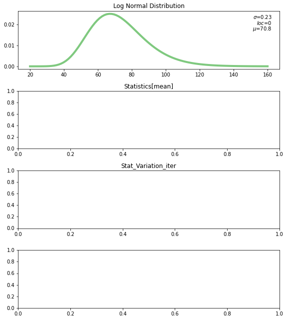
lnv = LogNormVisualizer(0.23, 0, 70.8)
---------------------------------------------------------------------------
TypeError                                 Traceback (most recent call last)
<ipython-input-26-34708152cec1> in <module>
----> 1 lnv = LogNormVisualizer(0.23, 0, 70.8)

<ipython-input-25-7235e5af6dae> in __init__(self, shape, loc, median, xs)
     93         self.r_max = None
     94         self.df = pd.DataFrame(columns=['n', 'iters', 'kind','mean_d','std_d'])
---> 95         self.update_rv()
     96         self.link_widgets()
     97

<ipython-input-25-7235e5af6dae> in update_rv(self)
    233 #         self.w_rv.clear_output()
    234         self.update_rv_plot()
--> 235         self.update_stat_plot()
    236         self.update_var_plot()
    237

<ipython-input-25-7235e5af6dae> in update_stat_plot(self)
    190         self.ax2.clear()
    191         self.ax2.set_title(f"Statistics[{self.w_kind.value}]")
--> 192         self.sample_d = computing_sampling_distribution(self.rv, self.w_n.value,
    193                                                        self.w_iters.value,
    194                                                        kind=self.w_kind.value)

TypeError: computing_sampling_distribution() got an unexpected keyword argument 'kind'
lnv.rv.mean(), lnv.rv.std()
# df = lnv.df
# df.loc[df.shape[0]] = [1,2,3,4]; df
lnv.view()
---------------------------------------------------------------------------
NameError                                 Traceback (most recent call last)
<ipython-input-27-73bcf06dbfee> in <module>
----> 1 lnv.view()

NameError: name 'lnv' is not defined
# lnv.df[lnv.df.kind=='mean'].plot.scatter(x='n',y='std_d',  ax=lnv.ax3)
lnv.df[lnv.df.kind=='mean'].plot.scatter(x='n',y='std_d', s='mean_d', ax=lnv.ax3)
# lnv.df
np.percentile?
# plt.xlim?
w = widgets.IntText()
l = widgets.IntText()
t = 2
def handle_change(change):
    t = change.new
    l.value = t

w.observe(handle_change, "value")
widgets.VBox([w,l])
# widgets.Label?
# display?
Estimating PI Computationally
Area of circle => \(\pi r^2\)
Area of square of size 2r => 4r^2
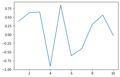
rv = stats.uniform(-1,2)
%matplotlib inline
plt.plot(np.linspace(1,10,10), rv.rvs(10))
plt.show()
@interact
def estimate_pi(n=(1,1000000)):
    x = stats.uniform(-1,2)
    y = stats.uniform(-1,2)
    dist = np.sqrt( x.rvs(n)**2+y.rvs(n)**2)
#     print(dist[:5])
    in_circle = dist <= 1
    pi = sum(in_circle)*4/n
    return pi
#     print(f"Estimated PI {pi} with n:{n}")
s = [estimate_pi(10000) for trials in range(1000)]
sample = np.array(s)
plt.hist(sample, bins=40)
plt.show()
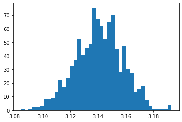
sample.mean(), sample.std(), np.percentile(sample, [5,95])
(3.1407156, 0.017060112445115943, array([3.1116 , 3.16882]))
Part 2
What if we don’t know the underlying assumption?
Take the Sample
Generate Model for Population from Sample
Calculate Sampling Statistics by running experiments on this model
sample = [1,2,3,4,5,2,1 ,4]
n = len(sample)
np.random.choice(sample,
                 n,
                 replace=True) # New sample from original sample , after this you can run experiment and calculate sampling statistics
array([4, 1, 1, 3, 2, 5, 5, 5])
Resampling
class Resampler(object):
def __init__(self, sample, xlim=None, iters=1000):
self.sample = sample
self.n = len(sample)
self.iters = iters
def resample(self):
new_sample = np.random.choice(self.sample, self.n, replace=True)
return new_sample
def sample_stat(self, sample):
return sample.mean()
def computing_sampling_distribution(self):
stats = [self.sample_stat(self.resample()) for i in range(self.iters)]
return np.array(stats)
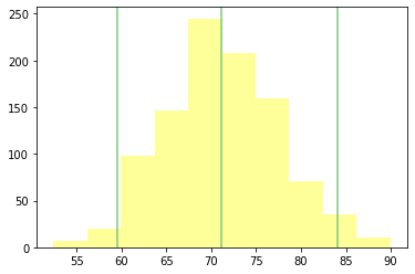
def plot_summary_statistics_distribution(self):
fig, ax = plt.subplots(1)
stats = self.computing_sampling_distribution()
mean = stats.mean()
SE = stats.std()
conf_int = np.percentile(stats, [2.5, 97.5]) # 95% confidence interval
plt.axvline(mean, color=COLOR1)
plt.axvline(conf_int[0], color=COLOR1)
plt.axvline(conf_int[1], color=COLOR1)
# plt.xlim(mean-4std, )
plt.hist(stats, color=COLOR4)
plt.show()
# s = np.random.random([1, 100]).flatten()
s = weight.rvs(10)
rsample = Resampler(s, iters=1000)
rsample.sample.shape
(10,)
# stat = rsample.computing_sampling_distribution()
# stat.shape
rsample.plot_summary_statistics_distribution()
np.random.choice([1,2,3],3, replace=True)
array([3, 1, 3])
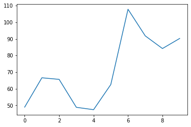
plt.plot(s)
[<matplotlib.lines.Line2D at 0x7feaabb10430>]
xs = np.linspace(20, 160, 100)
plt.plot(weight.pdf(xs))
[<matplotlib.lines.Line2D at 0x7feaabc22d60>]
type(weight)
scipy.stats._distn_infrastructure.rv_frozen
type(sample)
list
class StdResampler(Resampler):
    def sample_stat(self, sample):
        return sample.std()
s = weight.rvs(1000)
rsample = StdResampler(s, iters=1000)
rsample.sample.shape
(1000,)
rsample.plot_summary_statistics_distribution()
Part 3
In this section we will implement above for multiple group problems
mu1, sig1 = 178, 7.7
male_height = stats.norm(mu1, sig1); male_height
<scipy.stats._distn_infrastructure.rv_frozen at 0x7feaab9c58e0>
mu2, sig2 = 163, 7.3
female_height = stats.norm(mu2, sig2); female_height
<scipy.stats._distn_infrastructure.rv_frozen at 0x7feaab9ec4c0>
n = 1000
male_sample = male_height.rvs(1000)
female_sample = female_height.rvs(1000)
male_mean = male_height.mean()
female_mean = female_height.mean()
male_std = male_height.std()
female_std = female_height.std()
difference = (mu1 - mu2)

relative_difference_by_male = difference/mu1*100
relative_difference_by_female = difference/mu2*100
relative_difference_by_male, relative_difference_by_female
(8.426966292134832, 9.202453987730062)
thresh = (male_mean*female_std+female_mean*male_std)/(male_std+female_std); thresh
170.3
male_overlap = sum((male_sample < thresh))/ len(male_sample)
male_overlap
0.163
female_overlap = sum((female_sample > thresh))/ len(female_sample);
female_overlap
0.139
overlap = (male_overlap + female_overlap)/2; overlap
0.15100000000000002
prob_superiority = sum(male_sample > female_sample)/(len(male_sample)+len(female_sample))
prob_superiority = (male_sample > female_sample).mean()
prob_superiority
0.929
def overlap(grp1_sample, grp2_sample):
    """
        grp1: Control
        grp2: Treatment
    """

#     grp1_sample = grp1.rvs(1000)
#     grp2_sample = grp2.rvs(1000)
    m1 = grp1_sample.mean()  #grp1.mean()
    m2 = grp2_sample.mean()  #grp2.mean()
    s1 = grp1_sample.std()  #grp1.std()
    s2 = grp2_sample.std()  #grp1.std()
    thresh = (m1*s2+m2*s1)/(s1+s2)

    grp1_overlap = sum(grp1_sample<thresh)/ len(grp1_sample)
    grp2_overlap = sum(grp2_sample>thresh)/ len(grp2_sample)
    misclassification_rate = (grp1_overlap+grp2_overlap)/2
    return misclassification_rate
grp1_sample = male_height.rvs(1000)
grp2_sample = female_height.rvs(1000)

overlap(grp1_sample, grp2_sample)
0.166
def prob_superior(grp1_sample, grp2_sample):
    # Assumes same size
    assert len(grp1_sample) == len(grp2_sample)
    return(grp1_sample>grp2_sample).mean()
prob_superior(grp1_sample, grp2_sample)
0.932
grp1_sample.var()
58.99469052969996
def cohen_effect(grp1_sample, grp2_sample):
    diff = grp1_sample.mean() - grp2_sample.mean()
    var1, var2 = grp1_sample.var(), grp2_sample.var()
    n1, n2 = len(grp1_sample), len(grp2_sample)
    pooled_var = (n1*var1+n2*var2)/(n1+n2)
    d = diff/np.sqrt(pooled_var)
    return d
cohen_effect(grp1_sample, grp2_sample)
1.9942476570475194
def color_data(inp, CI):
    a, b = CI
    t1 = inp< a
    t2= inp>b
    color_data = (t1+t2).astype(np.int)
    return color_data

class MultiGrpResampler(object):
    def __init__(self, sample1, sample2, xlim=None, iters=1000, summary_stat='cohen'):
        self.sample1 = sample1
        self.sample2 = sample2
        self.xlim = xlim
        self.iters = iters
        self.summary_stat = summary_stat

    def resample(self):
        new_sample1 = np.random.choice(self.sample1, len(self.sample1), replace=True)
        new_sample2 = np.random.choice(self.sample2, len(self.sample2), replace=True)
        return new_sample1, new_sample2

    def calc_summary_stat(self, sample1, sample2):
        if self.summary_stat == 'cohen':
            return cohen_effect(sample1, sample2)
        if self.summary_stat == 'overlap':
            return overlap(sample1, sample2)
        if self.summary_stat == 'prob_superiority':
            return prob_superior(sample1, sample2)


    def compute_sampling_distribution(self):
        summary_stats = [self.calc_summary_stat(*self.resample()) for i in range(self.iters)]
        return np.array(summary_stats)


    def sampling_distribution(self):
        summary_stats = self.compute_sampling_distribution()

        mean = summary_stats.mean()
        std = summary_stats.std()
        CI = np.percentile(summary_stats, [5, 95]) # 90% confidence interval

        return  summary_stats, mean, std, CI


    def plot_sampling_distribution(self):
        summary_stats, mean, std, CI = self.sampling_distribution()
        bins = 30
#         hist_data = np.histogram(summary_stats, bins)[1]
        x_sc = LinearScale()
        y_sc = LinearScale()
        col_sc = ColorScale(colors=['MediumSeaGreen', 'Red'])
        y,edges = np.histogram(summary_stats, bins)
        centers = 0.5*(edges[1:]+ edges[:-1])
        cdata = np.array(col_sc.colors)[color_data(centers, CI)].tolist()
        ax_x = Axis(scale=x_sc, tick_format='0.3f')
        ax_y = Axis(scale=y_sc, orientation='vertical')
        vline_mean = pltbq.vline(mean, stroke_width=2, colors=['orangered'], scales={'y': y_sc, 'x': x_sc, 'color': col_sc})
        vline_a = pltbq.vline(CI[0], stroke_width=2, colors=['steelblue'], scales={'y': y_sc, 'x': x_sc, 'color': col_sc})
        vline_b = pltbq.vline(CI[1], stroke_width=2, colors=['steelblue'], scales={'y': y_sc, 'x': x_sc, 'color': col_sc})
        hist = Hist(sample=summary_stats, scales={'sample': x_sc, 'count': y_sc, 'color': col_sc}, bins=bins, colors=cdata)
        fig = Figure(marks=[hist, vline_mean, vline_a, vline_b], axes=[ax_x, ax_y], padding=0,
                     title=f'Sampling Distribution {self.summary_stat}' )
#         print(fig.marks[0].colors)

        return fig
sample1 = male_height.rvs(1000)
sample2 = female_height.rvs(1000)

rsampl = MultiGrpResampler(sample1, sample2,)
summary_stats, mean, std, CI = rsampl.sampling_distribution()
mean, std, CI
(1.988103230980105, 0.05500478400582647, array([1.89740944, 2.07562714]))
def color_data(inp, CI):
    a, b = CI
    t1 = inp< a
    t2= inp>b
    color_data = (t1+t2).astype(np.int)
    return color_data
x_sc = LinearScale()
y_sc = LinearScale()
col_sc = ColorScale(colors=['MediumSeaGreen', 'Red'])
# hist = Hist(data=summary_stats, scales={'summary_statistics': x_sc, 'count':y_sc})

hist = Hist(sample=summary_stats, scales={'sample': x_sc, 'count': y_sc, 'color': col_sc})
len(hist.midpoints)
0
ax_x = Axis(scale=x_sc, tick_format='0.2f')
ax_y = Axis(scale=y_sc, orientation='vertical')
ax_x
Axis(scale=LinearScale(), tick_format='0.2f')
color_data(hist.midpoints, CI)
array([], dtype=int64)
np.array(col_sc.colors)[color_data(hist.midpoints, CI)].tolist()
[]
hist.bins = 30
hist.colors = np.array(col_sc.colors)[color_data(hist.midpoints, CI)].tolist()
hist.colors
[]
# Figure(marks=[hist], axes=[ax_x, ax_y], padding=0, title='Sampling Distribution' )
vline_mean = pltbq.vline(mean, stroke_width=2, colors=['orangered'], scales={'y': y_sc, 'x': x_sc})
vline_a = pltbq.vline(CI[0], stroke_width=2, colors=['steelblue'], scales={'y': y_sc, 'x': x_sc})
vline_b = pltbq.vline(CI[1], stroke_width=2, colors=['steelblue'], scales={'y': y_sc, 'x': x_sc})
vline_mean, vline_a, vline_b
(Lines(colors=['orangered'], interactions={'hover': 'tooltip'}, preserve_domain={'x': False, 'y': True}, scales={'y': LinearScale(allow_padding=False, max=1.0, min=0.0), 'x': LinearScale()}, scales_metadata={'x': {'orientation': 'horizontal', 'dimension': 'x'}, 'y': {'orientation': 'vertical', 'dimension': 'y'}, 'color': {'dimension': 'color'}}, tooltip_style={'opacity': 0.9}, x=array([2.12200944, 2.12200944]), y=array([0, 1])),
 Lines(colors=['steelblue'], interactions={'hover': 'tooltip'}, preserve_domain={'x': False, 'y': True}, scales={'y': LinearScale(allow_padding=False, max=1.0, min=0.0), 'x': LinearScale()}, scales_metadata={'x': {'orientation': 'horizontal', 'dimension': 'x'}, 'y': {'orientation': 'vertical', 'dimension': 'y'}, 'color': {'dimension': 'color'}}, tooltip_style={'opacity': 0.9}, x=array([2.02652263, 2.02652263]), y=array([0, 1])),
 Lines(colors=['steelblue'], interactions={'hover': 'tooltip'}, preserve_domain={'x': False, 'y': True}, scales={'y': LinearScale(allow_padding=False, max=1.0, min=0.0), 'x': LinearScale()}, scales_metadata={'x': {'orientation': 'horizontal', 'dimension': 'x'}, 'y': {'orientation': 'vertical', 'dimension': 'y'}, 'color': {'dimension': 'color'}}, tooltip_style={'opacity': 0.9}, x=array([2.21439821, 2.21439821]), y=array([0, 1])))
Figure(marks=[hist, vline_mean, vline_a, vline_b], axes=[ax_x, ax_y], padding=0, title='Sampling Distribution 2' )
Function Call
bins=30
y,edges = np.histogram(summary_stats, bins)
centers = 0.5*(edges[1:]+ edges[:-1])
cdata = np.array(col_sc.colors)[color_data(centers, CI)].tolist()
cdata
['Red',
 'Red',
 'Red',
 'Red',
 'Red',
 'Red',
 'Red',
 'Red',
 'MediumSeaGreen',
 'MediumSeaGreen',
 'MediumSeaGreen',
 'MediumSeaGreen',
 'MediumSeaGreen',
 'MediumSeaGreen',
 'MediumSeaGreen',
 'MediumSeaGreen',
 'MediumSeaGreen',
 'MediumSeaGreen',
 'MediumSeaGreen',
 'MediumSeaGreen',
 'MediumSeaGreen',
 'MediumSeaGreen',
 'Red',
 'Red',
 'Red',
 'Red',
 'Red',
 'Red',
 'Red',
 'Red']
n = 100000
sample1 = male_height.rvs(n)
sample2 = female_height.rvs(1000)

rsampl = MultiGrpResampler(sample1, sample2,summary_stat='cohen')
fig = rsampl.plot_sampling_distribution()
# fig.marks[0].colors = cdata
fig
fig.marks[0]
Hist(bins=30, colors=['Red', 'Red', 'Red', 'Red', 'Red', 'Red', 'Red', 'MediumSeaGreen', 'MediumSeaGreen', 'MediumSeaGreen', 'MediumSeaGreen', 'MediumSeaGreen', 'MediumSeaGreen', 'MediumSeaGreen', 'MediumSeaGreen', 'MediumSeaGreen', 'MediumSeaGreen', 'MediumSeaGreen', 'MediumSeaGreen', 'MediumSeaGreen', 'MediumSeaGreen', 'MediumSeaGreen', 'Red', 'Red', 'Red', 'Red', 'Red', 'Red', 'Red', 'Red', 'Red'], interactions={'hover': 'tooltip'}, scales={'sample': LinearScale(), 'count': LinearScale(), 'color': ColorScale(colors=['MediumSeaGreen', 'Red'])}, scales_metadata={'sample': {'orientation': 'horizontal', 'dimension': 'x'}, 'count': {'orientation': 'vertical', 'dimension': 'y'}}, tooltip_style={'opacity': 0.9})
fig.marks[0].bins
30
fig
summary_stat = 'cohen'
summary_stats, mean, std, CI = rsampl.sampling_distribution()
x_sc = LinearScale()
y_sc = LinearScale()
col_sc = ColorScale(colors=['MediumSeaGreen', 'Red'])
ax_x = Axis(scale=x_sc, tick_format='0.2f')
ax_y = Axis(scale=y_sc, orientation='vertical')
hist = Hist(sample=summary_stats, scales={'sample': x_sc, 'count': y_sc, 'color': col_sc}, bins=30)
hist.colors
['steelblue']
vline_mean = pltbq.vline(mean, stroke_width=2, colors=['orangered'], scales={'y': y_sc, 'x': x_sc})
vline_a = pltbq.vline(CI[0], stroke_width=2, colors=['steelblue'], scales={'y': y_sc, 'x': x_sc})
vline_b = pltbq.vline(CI[1], stroke_width=2, colors=['steelblue'], scales={'y': y_sc, 'x': x_sc})
fig = Figure(marks=[hist, vline_mean, vline_a, vline_b], axes=[ax_x, ax_y], padding=0,
             title=f'Sampling Distribution {summary_stat}' )
fig
hist.bins = 30
hist.colors = np.array(col_sc.colors)[color_data(hist.midpoints, CI)].tolist()
hist.colors
[]
fig
summary_stat = 'cohen'
summary_stats, mean, std, CI = rsampl.sampling_distribution()
x_sc = LinearScale()
y_sc = LinearScale()
col_sc = ColorScale(colors=['MediumSeaGreen', 'Red'])
ax_x = Axis(scale=x_sc, tick_format='0.2f')
ax_y = Axis(scale=y_sc, orientation='vertical')
hist = Hist(sample=summary_stats, scales={'sample': x_sc, 'count': y_sc, 'color': col_sc}, bins=30)
# hist.bins = 30
with hist.hold_sync():
    hist.colors = np.array(col_sc.colors)[color_data(hist.midpoints, CI)].tolist()
vline_mean = pltbq.vline(mean, stroke_width=2, colors=['orangered'], scales={'y': y_sc, 'x': x_sc})
vline_a = pltbq.vline(CI[0], stroke_width=2, colors=['steelblue'], scales={'y': y_sc, 'x': x_sc})
vline_b = pltbq.vline(CI[1], stroke_width=2, colors=['steelblue'], scales={'y': y_sc, 'x': x_sc})
fig = Figure(marks=[hist, vline_mean, vline_a, vline_b], axes=[ax_x, ax_y], padding=0,
             title=f'Sampling Distribution {summary_stat}' )
fig
np.histogram([12,3,4,5, 19], bins=3)
(array([3, 1, 1]), array([ 3. , 8.33333333, 13.66666667, 19. ]))
np.histogram?