Introduction to Basic Customer Segmentation in Python
Problem
Exercise: Expedia Hotel Booking Dataset Customer Segmentation
Read more at kaggle
CEO : My board meeting is coming up next week. I need to present :-
A report of underperforming and overperforming segments
How to tailor the new marketing campaigns for different cities next month?
How to improve the user booking rate?
Imports
# import pandas as pd
# import numpy as np
# import scipy as sp
# import seaborn as sns
# import matplotlib as mpl
# import matplotlib.pyplot as plt

from fastai.basics import *
from nlphero.data.external import *
import sklearn as sk
import bqplot as bq
import seaborn as sns
import statsmodels.api as sm
from sklearn.preprocessing import StandardScaler
from sklearn.decomposition import PCA

from sklearn import metrics
from sklearn.cluster import KMeans
from scipy import stats
from ipywidgets import interact, interactive
Read The Data
# kaggle competitions download -c expedia-hotel-recommendations
path = untar_data("kaggle_competitions::expedia-hotel-recommendations"); path
Path('/Landmark2/pdo/.nlphero/data/expedia-hotel-recommendations')
path.ls()
(#4) [Path('/Landmark2/pdo/.nlphero/data/expedia-hotel-recommendations/sample_submission.csv'),Path('/Landmark2/pdo/.nlphero/data/expedia-hotel-recommendations/test.csv'),Path('/Landmark2/pdo/.nlphero/data/expedia-hotel-recommendations/train.csv'),Path('/Landmark2/pdo/.nlphero/data/expedia-hotel-recommendations/destinations.csv')]
df_train = pd.read_csv(path/"train.csv", parse_dates=['date_time', 'srch_ci', 'srch_co']); df_train.head()
| date_time | site_name | posa_continent | user_location_country | user_location_region | user_location_city | orig_destination_distance | user_id | is_mobile | is_package | ... | srch_children_cnt | srch_rm_cnt | srch_destination_id | srch_destination_type_id | is_booking | cnt | hotel_continent | hotel_country | hotel_market | hotel_cluster | |
|---|---|---|---|---|---|---|---|---|---|---|---|---|---|---|---|---|---|---|---|---|---|
| 0 | 2014-08-11 07:46:59 | 2 | 3 | 66 | 348 | 48862 | 2234.2641 | 12 | 0 | 1 | ... | 0 | 1 | 8250 | 1 | 0 | 3 | 2 | 50 | 628 | 1 |
| 1 | 2014-08-11 08:22:12 | 2 | 3 | 66 | 348 | 48862 | 2234.2641 | 12 | 0 | 1 | ... | 0 | 1 | 8250 | 1 | 1 | 1 | 2 | 50 | 628 | 1 |
| 2 | 2014-08-11 08:24:33 | 2 | 3 | 66 | 348 | 48862 | 2234.2641 | 12 | 0 | 0 | ... | 0 | 1 | 8250 | 1 | 0 | 1 | 2 | 50 | 628 | 1 |
| 3 | 2014-08-09 18:05:16 | 2 | 3 | 66 | 442 | 35390 | 913.1932 | 93 | 0 | 0 | ... | 0 | 1 | 14984 | 1 | 0 | 1 | 2 | 50 | 1457 | 80 |
| 4 | 2014-08-09 18:08:18 | 2 | 3 | 66 | 442 | 35390 | 913.6259 | 93 | 0 | 0 | ... | 0 | 1 | 14984 | 1 | 0 | 1 | 2 | 50 | 1457 | 21 |
5 rows × 24 columns
Basic Data Exploration
df_train.head().T
| 0 | 1 | 2 | 3 | 4 | |
|---|---|---|---|---|---|
| date_time | 2014-08-11 07:46:59 | 2014-08-11 08:22:12 | 2014-08-11 08:24:33 | 2014-08-09 18:05:16 | 2014-08-09 18:08:18 |
| site_name | 2 | 2 | 2 | 2 | 2 |
| posa_continent | 3 | 3 | 3 | 3 | 3 |
| user_location_country | 66 | 66 | 66 | 66 | 66 |
| user_location_region | 348 | 348 | 348 | 442 | 442 |
| user_location_city | 48862 | 48862 | 48862 | 35390 | 35390 |
| orig_destination_distance | 2234.26 | 2234.26 | 2234.26 | 913.193 | 913.626 |
| user_id | 12 | 12 | 12 | 93 | 93 |
| is_mobile | 0 | 0 | 0 | 0 | 0 |
| is_package | 1 | 1 | 0 | 0 | 0 |
| channel | 9 | 9 | 9 | 3 | 3 |
| srch_ci | 2014-08-27 | 2014-08-29 | 2014-08-29 | 2014-11-23 | 2014-11-23 |
| srch_co | 2014-08-31 | 2014-09-02 | 2014-09-02 | 2014-11-28 | 2014-11-28 |
| srch_adults_cnt | 2 | 2 | 2 | 2 | 2 |
| srch_children_cnt | 0 | 0 | 0 | 0 | 0 |
| srch_rm_cnt | 1 | 1 | 1 | 1 | 1 |
| srch_destination_id | 8250 | 8250 | 8250 | 14984 | 14984 |
| srch_destination_type_id | 1 | 1 | 1 | 1 | 1 |
| is_booking | 0 | 1 | 0 | 0 | 0 |
| cnt | 3 | 1 | 1 | 1 | 1 |
| hotel_continent | 2 | 2 | 2 | 2 | 2 |
| hotel_country | 50 | 50 | 50 | 50 | 50 |
| hotel_market | 628 | 628 | 628 | 1457 | 1457 |
| hotel_cluster | 1 | 1 | 1 | 80 | 21 |
df_train.info()
<class 'pandas.core.frame.DataFrame'>
RangeIndex: 37670293 entries, 0 to 37670292
Data columns (total 24 columns):
 #   Column                     Dtype
---  ------                     -----
 0   date_time                  datetime64[ns]
 1   site_name                  int64
 2   posa_continent             int64
 3   user_location_country      int64
 4   user_location_region       int64
 5   user_location_city         int64
 6   orig_destination_distance  float64
 7   user_id                    int64
 8   is_mobile                  int64
 9   is_package                 int64
 10  channel                    int64
 11  srch_ci                    object
 12  srch_co                    object
 13  srch_adults_cnt            int64
 14  srch_children_cnt          int64
 15  srch_rm_cnt                int64
 16  srch_destination_id        int64
 17  srch_destination_type_id   int64
 18  is_booking                 int64
 19  cnt                        int64
 20  hotel_continent            int64
 21  hotel_country              int64
 22  hotel_market               int64
 23  hotel_cluster              int64
dtypes: datetime64[ns](1), float64(1), int64(20), object(2)
memory usage: 6.7+ GB
!ls -la {path}
total 4414434
drwxrwxrwx+  2 ubuntu ubuntu          0 Oct 25 08:38 .
drwxrwxrwx+ 18 ubuntu ubuntu          0 Oct 25 08:38 ..
-rwxrwxrwx+  1 ubuntu ubuntu  138159416 Oct 25 08:38 destinations.csv
-rwxrwxrwx+  1 ubuntu ubuntu   31756066 Oct 25 08:38 sample_submission.csv
-rwxrwxrwx+  1 ubuntu ubuntu  276554476 Oct 25 08:38 test.csv
-rwxrwxrwx+  1 ubuntu ubuntu 4070445781 Oct 25 08:40 train.csv
len(df_train)
37670293
# df_train.describe()
Warning
Focus of this exersize is to learn about customer segmentation. We will start with a sample and come back to full dataset after formulating a methodology
Read Sample
df_sample = pd.read_csv("https://raw.githubusercontent.com/maoting1223/pycon_sg_2016/master/sample", parse_dates=['date_time', 'srch_ci', 'srch_co'], index_col=0)
df_sample.head().T
| 24636210 | 19837144 | 13066459 | 4691082 | 4878884 | |
|---|---|---|---|---|---|
| date_time | 2014-11-03 16:02:28 | 2013-03-13 19:25:01 | 2014-10-13 13:20:25 | 2013-11-05 10:40:34 | 2014-06-10 13:34:56 |
| site_name | 24 | 11 | 2 | 11 | 2 |
| posa_continent | 2 | 3 | 3 | 3 | 3 |
| user_location_country | 77 | 205 | 66 | 205 | 66 |
| user_location_region | 871 | 135 | 314 | 411 | 174 |
| user_location_city | 36643 | 38749 | 48562 | 52752 | 50644 |
| orig_destination_distance | 456.115 | 232.474 | 4468.27 | 171.602 | NaN |
| user_id | 792280 | 961995 | 495669 | 106611 | 596177 |
| is_mobile | 0 | 0 | 0 | 0 | 0 |
| is_package | 1 | 0 | 1 | 0 | 0 |
| channel | 1 | 9 | 9 | 0 | 9 |
| srch_ci | 2014-12-15 00:00:00 | 2013-03-13 00:00:00 | 2015-04-03 00:00:00 | 2013-11-07 00:00:00 | 2014-08-03 00:00:00 |
| srch_co | 2014-12-19 00:00:00 | 2013-03-14 00:00:00 | 2015-04-10 00:00:00 | 2013-11-08 00:00:00 | 2014-08-08 00:00:00 |
| srch_adults_cnt | 2 | 2 | 2 | 2 | 2 |
| srch_children_cnt | 0 | 0 | 0 | 0 | 1 |
| srch_rm_cnt | 1 | 1 | 1 | 1 | 1 |
| srch_destination_id | 8286 | 1842 | 8746 | 6210 | 12812 |
| srch_destination_type_id | 1 | 3 | 1 | 3 | 5 |
| is_booking | 0 | 0 | 0 | 1 | 0 |
| cnt | 1 | 1 | 1 | 1 | 1 |
| hotel_continent | 0 | 2 | 6 | 2 | 2 |
| hotel_country | 63 | 198 | 105 | 198 | 50 |
| hotel_market | 1258 | 786 | 29 | 1234 | 368 |
| hotel_cluster | 68 | 37 | 22 | 42 | 83 |
EDA-Descriptive Statistics
Basics
df_sample.info()
<class 'pandas.core.frame.DataFrame'>
Int64Index: 100000 entries, 24636210 to 1792721
Data columns (total 24 columns):
 #   Column                     Non-Null Count   Dtype
---  ------                     --------------   -----
 0   date_time                  100000 non-null  datetime64[ns]
 1   site_name                  100000 non-null  int64
 2   posa_continent             100000 non-null  int64
 3   user_location_country      100000 non-null  int64
 4   user_location_region       100000 non-null  int64
 5   user_location_city         100000 non-null  int64
 6   orig_destination_distance  63915 non-null   float64
 7   user_id                    100000 non-null  int64
 8   is_mobile                  100000 non-null  int64
 9   is_package                 100000 non-null  int64
 10  channel                    100000 non-null  int64
 11  srch_ci                    99878 non-null   datetime64[ns]
 12  srch_co                    99878 non-null   datetime64[ns]
 13  srch_adults_cnt            100000 non-null  int64
 14  srch_children_cnt          100000 non-null  int64
 15  srch_rm_cnt                100000 non-null  int64
 16  srch_destination_id        100000 non-null  int64
 17  srch_destination_type_id   100000 non-null  int64
 18  is_booking                 100000 non-null  int64
 19  cnt                        100000 non-null  int64
 20  hotel_continent            100000 non-null  int64
 21  hotel_country              100000 non-null  int64
 22  hotel_market               100000 non-null  int64
 23  hotel_cluster              100000 non-null  int64
dtypes: datetime64[ns](3), float64(1), int64(20)
memory usage: 19.1 MB
Attention
Almost a third of
orig_destination_distanceis missingSome rows are missing in srch_ci & srch_co. [~122]
df_sample.describe().T
| count | mean | std | min | 25% | 50% | 75% | max | |
|---|---|---|---|---|---|---|---|---|
| site_name | 100000.0 | 9.838570 | 11.996426 | 2.0000 | 2.0000 | 2.0000 | 15.00000 | 5.300000e+01 |
| posa_continent | 100000.0 | 2.678150 | 0.749018 | 0.0000 | 3.0000 | 3.0000 | 3.00000 | 4.000000e+00 |
| user_location_country | 100000.0 | 85.995070 | 59.292002 | 0.0000 | 66.0000 | 66.0000 | 70.00000 | 2.390000e+02 |
| user_location_region | 100000.0 | 308.636990 | 208.706581 | 0.0000 | 174.0000 | 314.0000 | 385.00000 | 1.025000e+03 |
| user_location_city | 100000.0 | 27676.391240 | 16768.647409 | 0.0000 | 12949.0000 | 27655.0000 | 42328.00000 | 5.650700e+04 |
| orig_destination_distance | 63915.0 | 1960.661721 | 2228.153377 | 0.0056 | 312.7921 | 1131.8353 | 2542.35935 | 1.196538e+04 |
| user_id | 100000.0 | 605438.332130 | 351615.377136 | 14.0000 | 298796.2500 | 602882.5000 | 915722.25000 | 1.198783e+06 |
| is_mobile | 100000.0 | 0.133770 | 0.340407 | 0.0000 | 0.0000 | 0.0000 | 0.00000 | 1.000000e+00 |
| is_package | 100000.0 | 0.248140 | 0.431936 | 0.0000 | 0.0000 | 0.0000 | 0.00000 | 1.000000e+00 |
| channel | 100000.0 | 5.858590 | 3.722823 | 0.0000 | 2.0000 | 9.0000 | 9.00000 | 1.000000e+01 |
| srch_adults_cnt | 100000.0 | 2.020710 | 0.909774 | 0.0000 | 2.0000 | 2.0000 | 2.00000 | 9.000000e+00 |
| srch_children_cnt | 100000.0 | 0.336750 | 0.734449 | 0.0000 | 0.0000 | 0.0000 | 0.00000 | 9.000000e+00 |
| srch_rm_cnt | 100000.0 | 1.111750 | 0.451602 | 0.0000 | 1.0000 | 1.0000 | 1.00000 | 8.000000e+00 |
| srch_destination_id | 100000.0 | 14426.327380 | 11036.981220 | 4.0000 | 8267.0000 | 9145.0000 | 18784.00000 | 6.503500e+04 |
| srch_destination_type_id | 100000.0 | 2.577290 | 2.149263 | 1.0000 | 1.0000 | 1.0000 | 5.00000 | 9.000000e+00 |
| is_booking | 100000.0 | 0.079930 | 0.271186 | 0.0000 | 0.0000 | 0.0000 | 0.00000 | 1.000000e+00 |
| cnt | 100000.0 | 1.487980 | 1.280262 | 1.0000 | 1.0000 | 1.0000 | 2.00000 | 1.200000e+02 |
| hotel_continent | 100000.0 | 3.150920 | 1.620534 | 0.0000 | 2.0000 | 2.0000 | 4.00000 | 6.000000e+00 |
| hotel_country | 100000.0 | 81.093290 | 56.111519 | 0.0000 | 50.0000 | 50.0000 | 106.00000 | 2.120000e+02 |
| hotel_market | 100000.0 | 598.848330 | 510.959297 | 0.0000 | 158.0000 | 591.0000 | 701.00000 | 2.117000e+03 |
| hotel_cluster | 100000.0 | 49.860370 | 28.885423 | 0.0000 | 25.0000 | 49.0000 | 73.00000 | 9.900000e+01 |
df_sample['user_location_region'].nunique()
779
df_sample['user_location_city'].nunique()
10779
df_sample['date_time'].min(), df_sample['date_time'].max()
(Timestamp('2013-01-07 00:33:47'), Timestamp('2014-12-31 23:47:14'))
df_sample['srch_ci'].min(), df_sample['srch_ci'].max()
(Timestamp('2013-01-07 00:00:00'), Timestamp('2016-05-10 00:00:00'))
df_sample['srch_co'].min(), df_sample['srch_co'].max()
(Timestamp('2013-01-08 00:00:00'), Timestamp('2016-05-13 00:00:00'))
df_sample.nunique()
date_time                    99886
site_name                       41
posa_continent                   5
user_location_country          201
user_location_region           779
user_location_city           10779
orig_destination_distance    62206
user_id                      88863
is_mobile                        2
is_package                       2
channel                         11
srch_ci                       1066
srch_co                       1068
srch_adults_cnt                 10
srch_children_cnt               10
srch_rm_cnt                      9
srch_destination_id           8827
srch_destination_type_id         8
is_booking                       2
cnt                             32
hotel_continent                  7
hotel_country                  178
hotel_market                  1843
hotel_cluster                  100
dtype: int64
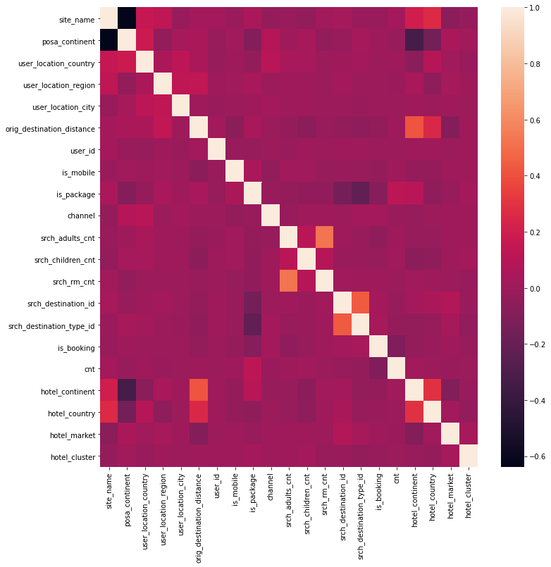
Correlation
Correlation between booking and hotel room
pd.crosstab(df_sample['is_booking'], df_sample['srch_rm_cnt'])
| srch_rm_cnt | 0 | 1 | 2 | 3 | 4 | 5 | 6 | 7 | 8 |
|---|---|---|---|---|---|---|---|---|---|
| is_booking | |||||||||
| 0 | 0 | 84425 | 6091 | 975 | 253 | 108 | 61 | 29 | 65 |
| 1 | 1 | 7248 | 580 | 102 | 42 | 9 | 6 | 1 | 4 |
df_sample.groupby('srch_rm_cnt')['is_booking'].mean()
srch_rm_cnt
0    1.000000
1    0.079064
2    0.086943
3    0.094708
4    0.142373
5    0.076923
6    0.089552
7    0.033333
8    0.057971
Name: is_booking, dtype: float64
df_sample.groupby('srch_rm_cnt')['is_booking'].value_counts()
srch_rm_cnt  is_booking
0            1                 1
1            0             84425
             1              7248
2            0              6091
             1               580
3            0               975
             1               102
4            0               253
             1                42
5            0               108
             1                 9
6            0                61
             1                 6
7            0                29
             1                 1
8            0                65
             1                 4
Name: is_booking, dtype: int64
df_sample.groupby('srch_rm_cnt')['is_booking'].mean()
srch_rm_cnt
0    1.000000
1    0.079064
2    0.086943
3    0.094708
4    0.142373
5    0.076923
6    0.089552
7    0.033333
8    0.057971
Name: is_booking, dtype: float64
df_sample.corr()
| site_name | posa_continent | user_location_country | user_location_region | user_location_city | orig_destination_distance | user_id | is_mobile | is_package | channel | ... | srch_children_cnt | srch_rm_cnt | srch_destination_id | srch_destination_type_id | is_booking | cnt | hotel_continent | hotel_country | hotel_market | hotel_cluster | |
|---|---|---|---|---|---|---|---|---|---|---|---|---|---|---|---|---|---|---|---|---|---|
| site_name | 1.000000 | -0.637743 | 0.159283 | 0.130818 | -0.013471 | 0.027609 | 0.030404 | -0.005418 | 0.048820 | -0.027780 | ... | -0.031962 | 0.016585 | 0.034895 | -0.006934 | -0.013460 | 0.022274 | 0.201760 | 0.263167 | -0.068316 | -0.026689 |
| posa_continent | -0.637743 | 1.000000 | 0.179726 | -0.034647 | 0.039227 | 0.049808 | -0.015209 | 0.016331 | -0.093459 | 0.089680 | ... | 0.034453 | -0.033712 | -0.015535 | 0.037172 | 0.013319 | -0.018952 | -0.333578 | -0.156578 | 0.049214 | 0.018297 |
| user_location_country | 0.159283 | 0.179726 | 1.000000 | 0.058496 | 0.122686 | 0.047689 | -0.021091 | 0.003728 | -0.025284 | 0.109999 | ... | 0.037101 | 0.000858 | 0.013486 | 0.028888 | 0.001284 | 0.003539 | -0.063744 | 0.097624 | 0.015569 | -0.011876 |
| user_location_region | 0.130818 | -0.034647 | 0.058496 | 1.000000 | 0.132457 | 0.136560 | 0.002225 | 0.016982 | 0.040482 | -0.001600 | ... | 0.014009 | 0.000254 | 0.022567 | 0.001376 | 0.000253 | -0.007570 | 0.043027 | -0.050301 | 0.040367 | 0.004984 |
| user_location_city | -0.013471 | 0.039227 | 0.122686 | 0.132457 | 1.000000 | 0.014178 | -0.007989 | -0.003741 | 0.013032 | 0.023497 | ... | 0.002638 | -0.000694 | 0.000786 | -0.004399 | -0.002655 | -0.002175 | 0.007759 | -0.001987 | 0.008558 | 0.000102 |
| orig_destination_distance | 0.027609 | 0.049808 | 0.047689 | 0.136560 | 0.014178 | 1.000000 | 0.017015 | -0.059464 | 0.041991 | -0.000398 | ... | -0.059722 | -0.012484 | -0.036314 | -0.042859 | -0.033480 | 0.009483 | 0.416180 | 0.254321 | -0.090112 | 0.003624 |
| user_id | 0.030404 | -0.015209 | -0.021091 | 0.002225 | -0.007989 | 0.017015 | 1.000000 | -0.011439 | -0.018901 | -0.003593 | ... | 0.002983 | -0.001625 | 0.002716 | 0.007133 | 0.001561 | 0.001355 | 0.002447 | 0.008707 | -0.002463 | 0.003202 |
| is_mobile | -0.005418 | 0.016331 | 0.003728 | 0.016982 | -0.003741 | -0.059464 | -0.011439 | 1.000000 | 0.046903 | -0.030770 | ... | 0.018211 | -0.022565 | -0.007140 | -0.016039 | -0.028623 | 0.008084 | -0.024144 | -0.029574 | 0.007644 | 0.012145 |
| is_package | 0.048820 | -0.093459 | -0.025284 | 0.040482 | 0.013032 | 0.041991 | -0.018901 | 0.046903 | 1.000000 | -0.011269 | ... | -0.037673 | -0.036653 | -0.146647 | -0.224422 | -0.081307 | 0.126500 | 0.108993 | -0.044426 | -0.014636 | 0.031399 |
| channel | -0.027780 | 0.089680 | 0.109999 | -0.001600 | 0.023497 | -0.000398 | -0.003593 | -0.030770 | -0.011269 | 1.000000 | ... | 0.004202 | 0.010191 | -0.000392 | 0.021612 | 0.025697 | -0.010248 | -0.022241 | -0.001217 | 0.006164 | 0.002596 |
| srch_adults_cnt | -0.013405 | 0.012350 | 0.042526 | 0.005487 | 0.006628 | -0.024039 | -0.007370 | 0.016661 | -0.024097 | -0.014931 | ... | 0.107061 | 0.525970 | 0.005651 | -0.012119 | -0.046350 | 0.014024 | -0.019355 | -0.018169 | 0.010203 | 0.006482 |
| srch_children_cnt | -0.031962 | 0.034453 | 0.037101 | 0.014009 | 0.002638 | -0.059722 | 0.002983 | 0.018211 | -0.037673 | 0.004202 | ... | 1.000000 | 0.091711 | -0.008784 | -0.007217 | -0.023228 | 0.019242 | -0.061707 | -0.045921 | 0.005056 | 0.021477 |
| srch_rm_cnt | 0.016585 | -0.033712 | 0.000858 | 0.000254 | -0.000694 | -0.012484 | -0.001625 | -0.022565 | -0.036653 | 0.010191 | ... | 0.091711 | 1.000000 | 0.018139 | 0.013618 | 0.009454 | -0.000487 | 0.019150 | 0.011055 | 0.000104 | -0.012177 |
| srch_destination_id | 0.034895 | -0.015535 | 0.013486 | 0.022567 | 0.000786 | -0.036314 | 0.002716 | -0.007140 | -0.146647 | -0.000392 | ... | -0.008784 | 0.018139 | 1.000000 | 0.435605 | 0.027674 | -0.021947 | 0.030365 | 0.053862 | 0.081240 | -0.010406 |
| srch_destination_type_id | -0.006934 | 0.037172 | 0.028888 | 0.001376 | -0.004399 | -0.042859 | 0.007133 | -0.016039 | -0.224422 | 0.021612 | ... | -0.007217 | 0.013618 | 0.435605 | 1.000000 | 0.037398 | -0.024544 | -0.035655 | -0.021522 | 0.035783 | -0.033039 |
| is_booking | -0.013460 | 0.013319 | 0.001284 | 0.000253 | -0.002655 | -0.033480 | 0.001561 | -0.028623 | -0.081307 | 0.025697 | ... | -0.023228 | 0.009454 | 0.027674 | 0.037398 | 1.000000 | -0.108628 | -0.025629 | -0.004763 | 0.012633 | -0.018192 |
| cnt | 0.022274 | -0.018952 | 0.003539 | -0.007570 | -0.002175 | 0.009483 | 0.001355 | 0.008084 | 0.126500 | -0.010248 | ... | 0.019242 | -0.000487 | -0.021947 | -0.024544 | -0.108628 | 1.000000 | 0.020670 | 0.001443 | -0.008747 | -0.000607 |
| hotel_continent | 0.201760 | -0.333578 | -0.063744 | 0.043027 | 0.007759 | 0.416180 | 0.002447 | -0.024144 | 0.108993 | -0.022241 | ... | -0.061707 | 0.019150 | 0.030365 | -0.035655 | -0.025629 | 0.020670 | 1.000000 | 0.295991 | -0.096278 | -0.015632 |
| hotel_country | 0.263167 | -0.156578 | 0.097624 | -0.050301 | -0.001987 | 0.254321 | 0.008707 | -0.029574 | -0.044426 | -0.001217 | ... | -0.045921 | 0.011055 | 0.053862 | -0.021522 | -0.004763 | 0.001443 | 0.295991 | 1.000000 | 0.017868 | -0.025002 |
| hotel_market | -0.068316 | 0.049214 | 0.015569 | 0.040367 | 0.008558 | -0.090112 | -0.002463 | 0.007644 | -0.014636 | 0.006164 | ... | 0.005056 | 0.000104 | 0.081240 | 0.035783 | 0.012633 | -0.008747 | -0.096278 | 0.017868 | 1.000000 | 0.037060 |
| hotel_cluster | -0.026689 | 0.018297 | -0.011876 | 0.004984 | 0.000102 | 0.003624 | 0.003202 | 0.012145 | 0.031399 | 0.002596 | ... | 0.021477 | -0.012177 | -0.010406 | -0.033039 | -0.018192 | -0.000607 | -0.015632 | -0.025002 | 0.037060 | 1.000000 |
21 rows × 21 columns
fig, ax = plt.subplots(figsize=(12,12))
sns.heatmap(df_sample.corr(),ax =ax)
plt.show()
df_sample['srch_children_cnt'].corr(df_sample['is_booking'])
-0.023228499097508428
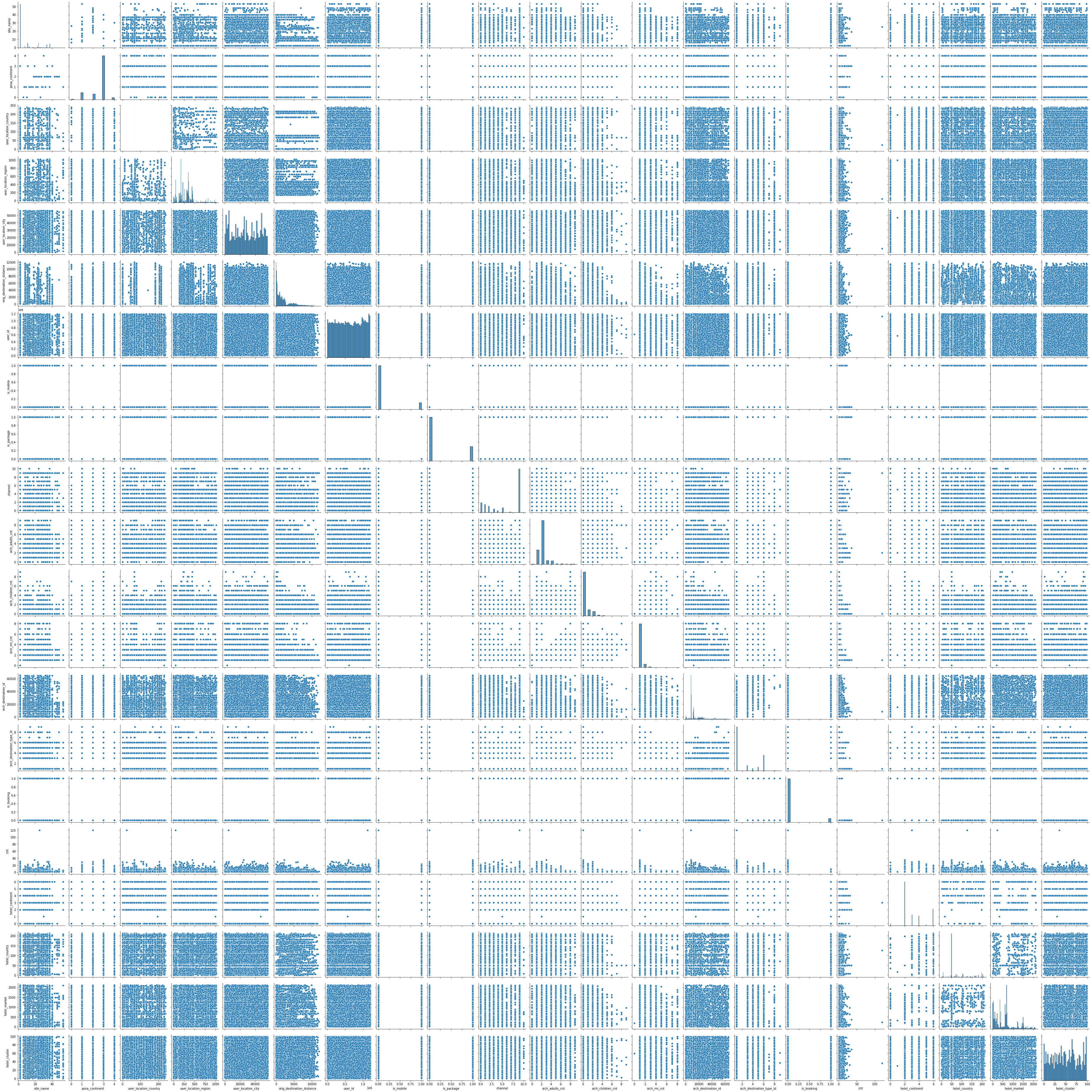
sns.pairplot(df_sample)
<seaborn.axisgrid.PairGrid at 0x7f34f56e0070>
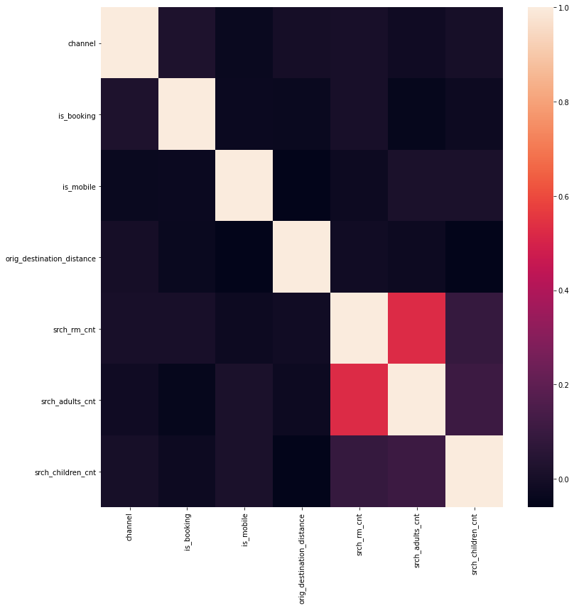
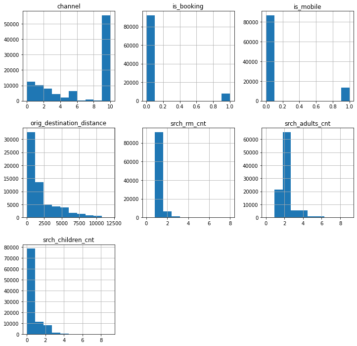
selection = ['channel', 'is_booking', 'is_mobile', 'orig_destination_distance', 'srch_rm_cnt', 'srch_adults_cnt', 'srch_children_cnt']
fig, axes = plt.subplots(nrows=1, ncols=1, figsize=(12,12)); axes
ax1 = axes
sns.heatmap(df_sample[selection].corr(),ax =ax1)
plt.tight_layout()
plt.show()
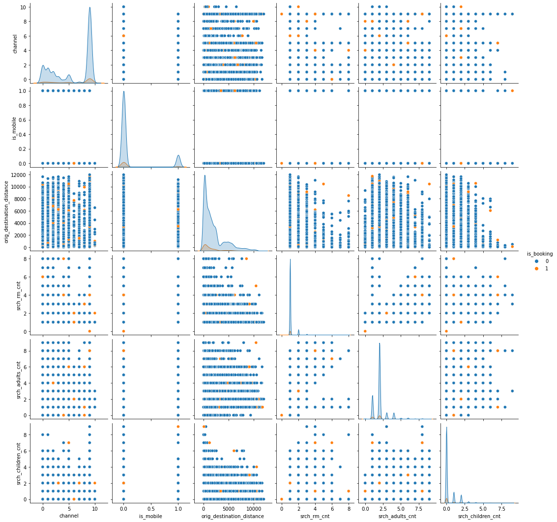
sns.pairplot(df_sample[selection], hue="is_booking", height=2.5)
<seaborn.axisgrid.PairGrid at 0x7f33e88640a0>
fig, ax = plt.subplots(1,1,figsize=(12,12))
df_sample[selection].hist(ax=fig.gca())
plt.show()
<ipython-input-73-88919a001020>:2: UserWarning: To output multiple subplots, the figure containing the passed axes is being cleared
  df_sample[selection].hist(ax=fig.gca())
# sns.kdeplot(df_sample[selection])
Distribution of number of Booking Attempts
df_userbooking = df_sample.groupby('user_id')['is_booking']\
.agg(number_of_booking='count').reset_index()
df_userbooking
| user_id | number_of_booking | |
|---|---|---|
| 0 | 14 | 1 |
| 1 | 38 | 1 |
| 2 | 40 | 1 |
| 3 | 156 | 2 |
| 4 | 160 | 1 |
| ... | ... | ... |
| 88858 | 1198722 | 1 |
| 88859 | 1198742 | 1 |
| 88860 | 1198748 | 1 |
| 88861 | 1198776 | 1 |
| 88862 | 1198783 | 2 |
88863 rows × 2 columns
df_sample = df_sample.merge(df_userbooking)
df_sample.head().T
| 0 | 1 | 2 | 3 | 4 | |
|---|---|---|---|---|---|
| date_time | 2014-11-03 16:02:28 | 2014-07-28 23:50:54 | 2013-03-13 19:25:01 | 2014-10-13 13:20:25 | 2013-11-05 10:40:34 |
| site_name | 24 | 24 | 11 | 2 | 11 |
| posa_continent | 2 | 2 | 3 | 3 | 3 |
| user_location_country | 77 | 77 | 205 | 66 | 205 |
| user_location_region | 871 | 871 | 135 | 314 | 411 |
| user_location_city | 36643 | 36643 | 38749 | 48562 | 52752 |
| orig_destination_distance | 456.115 | 454.461 | 232.474 | 4468.27 | 171.602 |
| user_id | 792280 | 792280 | 961995 | 495669 | 106611 |
| is_mobile | 0 | 0 | 0 | 0 | 0 |
| is_package | 1 | 1 | 0 | 1 | 0 |
| channel | 1 | 9 | 9 | 9 | 0 |
| srch_ci | 2014-12-15 00:00:00 | 2014-08-26 00:00:00 | 2013-03-13 00:00:00 | 2015-04-03 00:00:00 | 2013-11-07 00:00:00 |
| srch_co | 2014-12-19 00:00:00 | 2014-08-31 00:00:00 | 2013-03-14 00:00:00 | 2015-04-10 00:00:00 | 2013-11-08 00:00:00 |
| srch_adults_cnt | 2 | 1 | 2 | 2 | 2 |
| srch_children_cnt | 0 | 0 | 0 | 0 | 0 |
| srch_rm_cnt | 1 | 1 | 1 | 1 | 1 |
| srch_destination_id | 8286 | 8286 | 1842 | 8746 | 6210 |
| srch_destination_type_id | 1 | 1 | 3 | 1 | 3 |
| is_booking | 0 | 0 | 0 | 0 | 1 |
| cnt | 1 | 1 | 1 | 1 | 1 |
| hotel_continent | 0 | 0 | 2 | 6 | 2 |
| hotel_country | 63 | 63 | 198 | 105 | 198 |
| hotel_market | 1258 | 1258 | 786 | 29 | 1234 |
| hotel_cluster | 68 | 14 | 37 | 22 | 42 |
| number_of_booking | 2 | 2 | 1 | 1 | 2 |
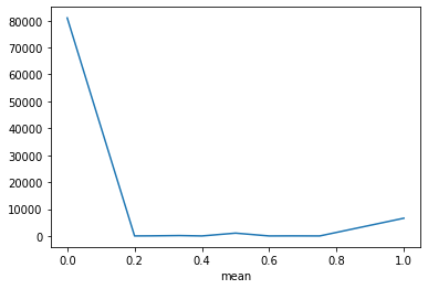
df_sample.groupby('user_id')['is_booking']\
.agg(['mean']).reset_index()\
.groupby('mean')['user_id']\
.agg('count')
mean
0.000000    80991
0.200000        5
0.250000       35
0.333333      153
0.400000        1
0.500000     1054
0.600000        1
0.666667       26
0.750000        1
1.000000     6596
Name: user_id, dtype: int64
(df_sample.groupby('user_id')['is_booking']\
.agg(['mean']).reset_index()\
.groupby('mean')['user_id']\
.agg('count')).plot(x='mean', y='user_id')
plt.show()
EDA-Business Rules Validation
Remove columns with zero occupant
pd.crosstab(df_sample['srch_adults_cnt'], df_sample['srch_children_cnt'])
| srch_children_cnt | 0 | 1 | 2 | 3 | 4 | 5 | 6 | 7 | 8 | 9 |
|---|---|---|---|---|---|---|---|---|---|---|
| srch_adults_cnt | ||||||||||
| 0 | 174 | 2 | 3 | 2 | 0 | 0 | 0 | 0 | 0 | 0 |
| 1 | 18749 | 2137 | 523 | 117 | 11 | 1 | 9 | 1 | 2 | 0 |
| 2 | 50736 | 7093 | 6529 | 972 | 208 | 14 | 7 | 1 | 0 | 0 |
| 3 | 3645 | 1131 | 469 | 131 | 27 | 5 | 2 | 2 | 0 | 2 |
| 4 | 3933 | 690 | 494 | 77 | 83 | 9 | 4 | 0 | 0 | 0 |
| 5 | 535 | 131 | 41 | 20 | 6 | 4 | 2 | 0 | 0 | 0 |
| 6 | 669 | 73 | 53 | 28 | 18 | 13 | 7 | 0 | 0 | 0 |
| 7 | 99 | 20 | 5 | 8 | 6 | 3 | 0 | 0 | 0 | 0 |
| 8 | 183 | 12 | 13 | 2 | 6 | 1 | 3 | 2 | 2 | 1 |
| 9 | 24 | 5 | 4 | 2 | 1 | 1 | 2 | 0 | 0 | 0 |
(df_sample['srch_adults_cnt']+df_sample['srch_children_cnt']) == 0
0        False
1        False
2        False
3        False
4        False
         ...
99995    False
99996    False
99997    False
99998    False
99999    False
Length: 100000, dtype: bool
df_sample = df_sample[(df_sample['srch_adults_cnt']+df_sample['srch_children_cnt']) > 0]

df_sample
| date_time | site_name | posa_continent | user_location_country | user_location_region | user_location_city | orig_destination_distance | user_id | is_mobile | is_package | ... | srch_rm_cnt | srch_destination_id | srch_destination_type_id | is_booking | cnt | hotel_continent | hotel_country | hotel_market | hotel_cluster | number_of_booking | |
|---|---|---|---|---|---|---|---|---|---|---|---|---|---|---|---|---|---|---|---|---|---|
| 0 | 2014-11-03 16:02:28 | 24 | 2 | 77 | 871 | 36643 | 456.1151 | 792280 | 0 | 1 | ... | 1 | 8286 | 1 | 0 | 1 | 0 | 63 | 1258 | 68 | 2 |
| 1 | 2014-07-28 23:50:54 | 24 | 2 | 77 | 871 | 36643 | 454.4611 | 792280 | 0 | 1 | ... | 1 | 8286 | 1 | 0 | 1 | 0 | 63 | 1258 | 14 | 2 |
| 2 | 2013-03-13 19:25:01 | 11 | 3 | 205 | 135 | 38749 | 232.4737 | 961995 | 0 | 0 | ... | 1 | 1842 | 3 | 0 | 1 | 2 | 198 | 786 | 37 | 1 |
| 3 | 2014-10-13 13:20:25 | 2 | 3 | 66 | 314 | 48562 | 4468.2720 | 495669 | 0 | 1 | ... | 1 | 8746 | 1 | 0 | 1 | 6 | 105 | 29 | 22 | 1 |
| 4 | 2013-11-05 10:40:34 | 11 | 3 | 205 | 411 | 52752 | 171.6021 | 106611 | 0 | 0 | ... | 1 | 6210 | 3 | 1 | 1 | 2 | 198 | 1234 | 42 | 2 |
| ... | ... | ... | ... | ... | ... | ... | ... | ... | ... | ... | ... | ... | ... | ... | ... | ... | ... | ... | ... | ... | ... |
| 99995 | 2013-03-31 16:45:01 | 2 | 3 | 66 | 351 | 21609 | 1386.4061 | 858268 | 0 | 0 | ... | 1 | 762 | 6 | 0 | 1 | 2 | 50 | 503 | 91 | 1 |
| 99996 | 2013-09-29 14:09:07 | 2 | 3 | 66 | 462 | 49272 | 698.1395 | 957708 | 0 | 0 | ... | 1 | 12843 | 5 | 0 | 1 | 2 | 50 | 661 | 6 | 1 |
| 99997 | 2014-07-11 22:05:54 | 37 | 1 | 69 | 998 | 52849 | NaN | 814512 | 1 | 1 | ... | 3 | 18773 | 1 | 0 | 1 | 6 | 22 | 1794 | 38 | 1 |
| 99998 | 2013-07-02 01:03:12 | 2 | 3 | 66 | 246 | 28491 | 207.2549 | 881704 | 0 | 1 | ... | 1 | 8859 | 1 | 0 | 1 | 2 | 50 | 212 | 89 | 1 |
| 99999 | 2014-12-19 19:59:12 | 11 | 3 | 205 | 354 | 53478 | 1198.4359 | 845482 | 0 | 0 | ... | 1 | 11848 | 1 | 0 | 1 | 2 | 50 | 705 | 42 | 1 |
99826 rows × 25 columns
Create a date column
df_sample.loc[:,'date'] =df_sample['date_time'].dt.date
df_sample.head().T
| 0 | 1 | 2 | 3 | 4 | |
|---|---|---|---|---|---|
| date_time | 2014-11-03 16:02:28 | 2014-07-28 23:50:54 | 2013-03-13 19:25:01 | 2014-10-13 13:20:25 | 2013-11-05 10:40:34 |
| site_name | 24 | 24 | 11 | 2 | 11 |
| posa_continent | 2 | 2 | 3 | 3 | 3 |
| user_location_country | 77 | 77 | 205 | 66 | 205 |
| user_location_region | 871 | 871 | 135 | 314 | 411 |
| user_location_city | 36643 | 36643 | 38749 | 48562 | 52752 |
| orig_destination_distance | 456.115 | 454.461 | 232.474 | 4468.27 | 171.602 |
| user_id | 792280 | 792280 | 961995 | 495669 | 106611 |
| is_mobile | 0 | 0 | 0 | 0 | 0 |
| is_package | 1 | 1 | 0 | 1 | 0 |
| channel | 1 | 9 | 9 | 9 | 0 |
| srch_ci | 2014-12-15 00:00:00 | 2014-08-26 00:00:00 | 2013-03-13 00:00:00 | 2015-04-03 00:00:00 | 2013-11-07 00:00:00 |
| srch_co | 2014-12-19 00:00:00 | 2014-08-31 00:00:00 | 2013-03-14 00:00:00 | 2015-04-10 00:00:00 | 2013-11-08 00:00:00 |
| srch_adults_cnt | 2 | 1 | 2 | 2 | 2 |
| srch_children_cnt | 0 | 0 | 0 | 0 | 0 |
| srch_rm_cnt | 1 | 1 | 1 | 1 | 1 |
| srch_destination_id | 8286 | 8286 | 1842 | 8746 | 6210 |
| srch_destination_type_id | 1 | 1 | 3 | 1 | 3 |
| is_booking | 0 | 0 | 0 | 0 | 1 |
| cnt | 1 | 1 | 1 | 1 | 1 |
| hotel_continent | 0 | 0 | 2 | 6 | 2 |
| hotel_country | 63 | 63 | 198 | 105 | 198 |
| hotel_market | 1258 | 1258 | 786 | 29 | 1234 |
| hotel_cluster | 68 | 14 | 37 | 22 | 42 |
| number_of_booking | 2 | 2 | 1 | 1 | 2 |
| date | 2014-11-03 | 2014-07-28 | 2013-03-13 | 2014-10-13 | 2013-11-05 |
df_sample.shape
(99826, 26)
Check booking date < check_in date < check out date
chk = df_sample[(df_sample['srch_ci']<df_sample['date']) |
          (df_sample['srch_co'] <df_sample['srch_ci'])]
chk.shape
(27, 26)
EDA - Create New Features
# duration

df_sample['duration'] = (df_sample['srch_co'] - df_sample['srch_ci'])/ np.timedelta64(1, "D")
df_sample['duration']
0        4.0
1        5.0
2        1.0
3        7.0
4        1.0
        ...
99995    4.0
99996    1.0
99997    7.0
99998    2.0
99999    3.0
Name: duration, Length: 99826, dtype: float64
df_sample.loc[df_sample['duration'] < 0, 'duration'] = np.nan
df_sample['days_in_advance'] = (df_sample['srch_ci'] - df_sample['date_time'])/  np.timedelta64(1, "D")
df_sample.loc[df_sample['days_in_advance'] < 0, 'days_in_advance'] = np.nan
df_sample.head().T
| 0 | 1 | 2 | 3 | 4 | |
|---|---|---|---|---|---|
| date_time | 2014-11-03 16:02:28 | 2014-07-28 23:50:54 | 2013-03-13 19:25:01 | 2014-10-13 13:20:25 | 2013-11-05 10:40:34 |
| site_name | 24 | 24 | 11 | 2 | 11 |
| posa_continent | 2 | 2 | 3 | 3 | 3 |
| user_location_country | 77 | 77 | 205 | 66 | 205 |
| user_location_region | 871 | 871 | 135 | 314 | 411 |
| user_location_city | 36643 | 36643 | 38749 | 48562 | 52752 |
| orig_destination_distance | 456.115 | 454.461 | 232.474 | 4468.27 | 171.602 |
| user_id | 792280 | 792280 | 961995 | 495669 | 106611 |
| is_mobile | 0 | 0 | 0 | 0 | 0 |
| is_package | 1 | 1 | 0 | 1 | 0 |
| channel | 1 | 9 | 9 | 9 | 0 |
| srch_ci | 2014-12-15 00:00:00 | 2014-08-26 00:00:00 | 2013-03-13 00:00:00 | 2015-04-03 00:00:00 | 2013-11-07 00:00:00 |
| srch_co | 2014-12-19 00:00:00 | 2014-08-31 00:00:00 | 2013-03-14 00:00:00 | 2015-04-10 00:00:00 | 2013-11-08 00:00:00 |
| srch_adults_cnt | 2 | 1 | 2 | 2 | 2 |
| srch_children_cnt | 0 | 0 | 0 | 0 | 0 |
| srch_rm_cnt | 1 | 1 | 1 | 1 | 1 |
| srch_destination_id | 8286 | 8286 | 1842 | 8746 | 6210 |
| srch_destination_type_id | 1 | 1 | 3 | 1 | 3 |
| is_booking | 0 | 0 | 0 | 0 | 1 |
| cnt | 1 | 1 | 1 | 1 | 1 |
| hotel_continent | 0 | 0 | 2 | 6 | 2 |
| hotel_country | 63 | 63 | 198 | 105 | 198 |
| hotel_market | 1258 | 1258 | 786 | 29 | 1234 |
| hotel_cluster | 68 | 14 | 37 | 22 | 42 |
| number_of_booking | 2 | 2 | 1 | 1 | 2 |
| date | 2014-11-03 | 2014-07-28 | 2013-03-13 | 2014-10-13 | 2013-11-05 |
| duration | 4 | 5 | 1 | 7 | 1 |
| days_in_advance | 41.3316 | 28.0063 | NaN | 171.444 | 1.55516 |
Underperforming and Overperforming Segments
Effect Size and Comparing to Mean
Here we are taking booking_rate per segment as our effect size.
df_sample.channel.nunique()
11
df_sample.columns
Index(['date_time', 'site_name', 'posa_continent', 'user_location_country',
       'user_location_region', 'user_location_city',
       'orig_destination_distance', 'user_id', 'is_mobile', 'is_package',
       'channel', 'srch_ci', 'srch_co', 'srch_adults_cnt', 'srch_children_cnt',
       'srch_rm_cnt', 'srch_destination_id', 'srch_destination_type_id',
       'is_booking', 'cnt', 'hotel_continent', 'hotel_country', 'hotel_market',
       'hotel_cluster', 'number_of_booking', 'date', 'duration',
       'days_in_advance'],
      dtype='object')
cat_list = ['site_name', 'posa_continent', 'user_location_country',
       'user_location_region', 'user_location_city','channel',
       'srch_destination_id', 'srch_destination_type_id',
       'hotel_continent', 'hotel_country', 'hotel_market',
       'hotel_cluster']
df_sample.groupby('channel')['is_booking']\
.agg(booking_rate='mean', num_of_bookings='sum')\
.reset_index()\
.sort_values(by='booking_rate')
| channel | booking_rate | num_of_bookings | |
|---|---|---|---|
| 7 | 7 | 0.043263 | 35 |
| 8 | 8 | 0.051852 | 14 |
| 3 | 3 | 0.060482 | 266 |
| 2 | 2 | 0.060583 | 474 |
| 6 | 6 | 0.068323 | 11 |
| 1 | 1 | 0.069568 | 713 |
| 0 | 0 | 0.072184 | 901 |
| 9 | 9 | 0.085365 | 4719 |
| 5 | 5 | 0.094533 | 581 |
| 4 | 4 | 0.120438 | 264 |
| 10 | 10 | 0.200000 | 3 |
@interact
def display_ranking(cat=cat_list):
    display(df_sample.groupby(cat)['is_booking']\
    .agg(booking_rate='mean', num_of_bookings='sum')\
    .reset_index()\
    .sort_values(by='booking_rate',  ascending=False))
## Population Booking Rate

df_sample['is_booking'].mean()
0.07994911145392984
Note
Looking at the data above we can see 4,5,9, 10 performing more than the population mean. However we need to ask the question are they really significant or just by chance?
Two Sample T-Test
Samples coming from 2 different group
Check each group for inference condition
Randomness
Independence n*p <= 10 n(1-p) <= 10
Normal
Sampled with Replacement
Sample size <= 10%N ( population)
Assign a signifance and confidence level ( for calculaing z*)
Calculate Confidence interval
\(CI = \hat{p}_1 - \hat{p}_1 \pm z^*\sqrt{ \frac{\hat{p}_1(1-\hat{p}_1)}{n_1}+ \frac{\hat{p}_2(1-\hat{p}_2)}{n_2}} \)
Calculate pvalue & t-test
df_sample.groupby('channel')['is_booking']\
    .agg(average='mean',
         bookings='count').reset_index()
| channel | average | bookings | |
|---|---|---|---|
| 0 | 0 | 0.072184 | 12482 |
| 1 | 1 | 0.069568 | 10249 |
| 2 | 2 | 0.060583 | 7824 |
| 3 | 3 | 0.060482 | 4398 |
| 4 | 4 | 0.120438 | 2192 |
| 5 | 5 | 0.094533 | 6146 |
| 6 | 6 | 0.068323 | 161 |
| 7 | 7 | 0.043263 | 809 |
| 8 | 8 | 0.051852 | 270 |
| 9 | 9 | 0.085365 | 55280 |
| 10 | 10 | 0.200000 | 15 |
def stat_comparison(cat, df):
    cat =  df.groupby(cat)['is_booking']\
                    .agg(sub_average='mean',
                         sub_bookings='count')\
                    .reset_index()

    cat['overall_average'] = df['is_booking'].mean()
    cat['overall_bookings'] = df['is_booking'].count()
    cat['rest_bookings'] = cat['overall_bookings']-cat['sub_bookings']
    cat['rest_average'] = (cat['overall_bookings']*cat['overall_average']- cat['sub_bookings']*cat['sub_average'])/cat['rest_bookings']

    cat['z_score'] = (cat['sub_average']-cat['rest_average'])/\
        np.sqrt(cat['overall_average']*(1-cat['overall_average'])
            *(1/cat['sub_bookings']+1/cat['rest_bookings']))

    cat['prob'] = np.around(stats.norm.cdf(cat['z_score']), decimals=10)


    def significant(x):
        if x >0.9:
            return 1
        elif x < 0.1:
            return -1
        else:
            return 0

    cat['significant'] = cat['prob'].apply(significant)
    return cat
stat_comparison('channel', df_sample)
| channel | sub_average | sub_bookings | overall_average | overall_bookings | rest_bookings | rest_average | z_score | prob | significant | |
|---|---|---|---|---|---|---|---|---|---|---|
| 0 | 0 | 0.072184 | 12482 | 0.079949 | 99826 | 87344 | 0.081059 | -3.419680 | 3.134747e-04 | -1 |
| 1 | 1 | 0.069568 | 10249 | 0.079949 | 99826 | 89577 | 0.081137 | -4.090773 | 2.149690e-05 | -1 |
| 2 | 2 | 0.060583 | 7824 | 0.079949 | 99826 | 92002 | 0.081596 | -6.579173 | 0.000000e+00 | -1 |
| 3 | 3 | 0.060482 | 4398 | 0.079949 | 99826 | 95428 | 0.080846 | -4.868548 | 5.621000e-07 | -1 |
| 4 | 4 | 0.120438 | 2192 | 0.079949 | 99826 | 97634 | 0.079040 | 7.067474 | 1.000000e+00 | 1 |
| 5 | 5 | 0.094533 | 6146 | 0.079949 | 99826 | 93680 | 0.078992 | 4.351672 | 9.999932e-01 | 1 |
| 6 | 6 | 0.068323 | 161 | 0.079949 | 99826 | 99665 | 0.079968 | -0.544360 | 2.930970e-01 | 0 |
| 7 | 7 | 0.043263 | 809 | 0.079949 | 99826 | 99017 | 0.080249 | -3.863018 | 5.599740e-05 | -1 |
| 8 | 8 | 0.051852 | 270 | 0.079949 | 99826 | 99556 | 0.080025 | -1.704595 | 4.413499e-02 | -1 |
| 9 | 9 | 0.085365 | 55280 | 0.079949 | 99826 | 44546 | 0.073228 | 7.028968 | 1.000000e+00 | 1 |
| 10 | 10 | 0.200000 | 15 | 0.079949 | 99826 | 99811 | 0.079931 | 1.714474 | 9.567791e-01 | 1 |
@interact
def review_stats(cat=cat_list):
    return stat_comparison(cat, df_sample)
Note
From above we can find significantly affected channel / cities/ region
Clustering - What are similar user cities?
Step1. What are the features I am going to use? (that makes sense)
What features may distinguish cities based on business sense and exploratory analysis
# Numerical Features
df_sample.columns
Index(['date_time', 'site_name', 'posa_continent', 'user_location_country',
       'user_location_region', 'user_location_city',
       'orig_destination_distance', 'user_id', 'is_mobile', 'is_package',
       'channel', 'srch_ci', 'srch_co', 'srch_adults_cnt', 'srch_children_cnt',
       'srch_rm_cnt', 'srch_destination_id', 'srch_destination_type_id',
       'is_booking', 'cnt', 'hotel_continent', 'hotel_country', 'hotel_market',
       'hotel_cluster', 'number_of_booking', 'date', 'duration',
       'days_in_advance'],
      dtype='object')
num_list = ['orig_destination_distance',  'is_mobile', 'is_package',
       'srch_adults_cnt', 'srch_children_cnt',
       'srch_rm_cnt', 'duration',
       'days_in_advance']

city_data = df_sample[['user_location_city']+num_list].dropna(axis=0)
city_data
| user_location_city | orig_destination_distance | is_mobile | is_package | srch_adults_cnt | srch_children_cnt | srch_rm_cnt | duration | days_in_advance | |
|---|---|---|---|---|---|---|---|---|---|
| 0 | 36643 | 456.1151 | 0 | 1 | 2 | 0 | 1 | 4.0 | 41.331620 |
| 1 | 36643 | 454.4611 | 0 | 1 | 1 | 0 | 1 | 5.0 | 28.006319 |
| 3 | 48562 | 4468.2720 | 0 | 1 | 2 | 0 | 1 | 7.0 | 171.444155 |
| 4 | 52752 | 171.6021 | 0 | 0 | 2 | 0 | 1 | 1.0 | 1.555162 |
| 5 | 54864 | 209.6633 | 0 | 0 | 1 | 0 | 1 | 3.0 | 6.484433 |
| ... | ... | ... | ... | ... | ... | ... | ... | ... | ... |
| 99993 | 36878 | 368.5449 | 0 | 0 | 1 | 0 | 1 | 1.0 | 9.359387 |
| 99995 | 21609 | 1386.4061 | 0 | 0 | 2 | 0 | 1 | 4.0 | 96.302072 |
| 99996 | 49272 | 698.1395 | 0 | 0 | 1 | 0 | 1 | 1.0 | 0.410336 |
| 99998 | 28491 | 207.2549 | 0 | 1 | 2 | 0 | 1 | 2.0 | 10.956111 |
| 99999 | 53478 | 1198.4359 | 0 | 0 | 2 | 1 | 1 | 3.0 | 11.167222 |
61554 rows × 9 columns
city_groups = city_data.groupby('user_location_city')\
.mean().reset_index().dropna(); city_groups
| user_location_city | orig_destination_distance | is_mobile | is_package | srch_adults_cnt | srch_children_cnt | srch_rm_cnt | duration | days_in_advance | |
|---|---|---|---|---|---|---|---|---|---|
| 0 | 0 | 2315.836250 | 0.000000 | 0.250000 | 1.750000 | 0.000000 | 1.000000 | 2.000000 | 77.959358 |
| 1 | 3 | 3451.384159 | 0.058824 | 0.294118 | 1.941176 | 0.470588 | 1.000000 | 4.294118 | 87.139739 |
| 2 | 7 | 5994.864000 | 0.000000 | 1.000000 | 2.000000 | 0.000000 | 1.000000 | 14.000000 | 57.287755 |
| 3 | 14 | 5342.819100 | 0.000000 | 0.000000 | 2.000000 | 0.750000 | 1.000000 | 7.000000 | 35.206548 |
| 4 | 21 | 2165.768900 | 0.000000 | 0.500000 | 1.500000 | 1.000000 | 1.000000 | 5.000000 | 30.946875 |
| ... | ... | ... | ... | ... | ... | ... | ... | ... | ... |
| 4480 | 56472 | 1394.624100 | 0.214286 | 0.357143 | 2.000000 | 0.285714 | 1.142857 | 3.285714 | 83.805879 |
| 4481 | 56488 | 5930.875650 | 0.000000 | 0.000000 | 1.500000 | 0.000000 | 1.000000 | 6.000000 | 130.960440 |
| 4482 | 56498 | 3288.597750 | 0.500000 | 0.500000 | 3.000000 | 1.000000 | 1.500000 | 4.500000 | 49.570741 |
| 4483 | 56505 | 1370.771600 | 1.000000 | 0.000000 | 2.000000 | 0.000000 | 1.000000 | 2.000000 | 22.968461 |
| 4484 | 56507 | 1941.016580 | 0.400000 | 0.600000 | 2.600000 | 0.400000 | 1.400000 | 5.000000 | 127.597354 |
4485 rows × 9 columns
Step2. Standardize the data
What is magnitude of data range ?
city_groups_std = city_groups.copy()
sc = StandardScaler()
city_groups_std.loc[:, num_list]= sc.fit_transform(city_groups_std[num_list])
city_groups_std
| user_location_city | orig_destination_distance | is_mobile | is_package | srch_adults_cnt | srch_children_cnt | srch_rm_cnt | duration | days_in_advance | |
|---|---|---|---|---|---|---|---|---|---|
| 0 | 0 | 0.295943 | -0.583534 | -0.030898 | -0.510201 | -0.684278 | -0.325406 | -0.676476 | 0.438680 |
| 1 | 3 | 0.997273 | -0.321107 | 0.112882 | -0.215089 | 0.183626 | -0.325406 | 0.417193 | 0.636132 |
| 2 | 7 | 2.568161 | -0.583534 | 2.413358 | -0.124285 | -0.684278 | -0.325406 | 5.044256 | -0.005927 |
| 3 | 14 | 2.165449 | -0.583534 | -0.845650 | -0.124285 | 0.698944 | -0.325406 | 1.707162 | -0.480852 |
| 4 | 21 | 0.203260 | -0.583534 | 0.783854 | -0.896118 | 1.160018 | -0.325406 | 0.753707 | -0.572470 |
| ... | ... | ... | ... | ... | ... | ... | ... | ... | ... |
| 4480 | 56472 | -0.273010 | 0.372450 | 0.318282 | -0.124285 | -0.157336 | 0.063454 | -0.063540 | 0.564427 |
| 4481 | 56488 | 2.528641 | -0.583534 | -0.845650 | -0.896118 | -0.684278 | -0.325406 | 1.230435 | 1.578633 |
| 4482 | 56498 | 0.896734 | 1.647094 | 0.783854 | 1.419380 | 1.160018 | 1.035602 | 0.515343 | -0.171906 |
| 4483 | 56505 | -0.287742 | 3.877723 | -0.845650 | -0.124285 | -0.684278 | -0.325406 | -0.676476 | -0.744070 |
| 4484 | 56507 | 0.064449 | 1.200969 | 1.109755 | 0.801914 | 0.053441 | 0.763400 | 0.753707 | 1.506299 |
4485 rows × 9 columns
km = KMeans(n_clusters=3, max_iter=300, random_state=None)
city_groups_std['cluster'] = km.fit_predict(city_groups_std[num_list])
city_groups_std
| user_location_city | orig_destination_distance | is_mobile | is_package | srch_adults_cnt | srch_children_cnt | srch_rm_cnt | duration | days_in_advance | cluster | |
|---|---|---|---|---|---|---|---|---|---|---|
| 0 | 0 | 0.295943 | -0.583534 | -0.030898 | -0.510201 | -0.684278 | -0.325406 | -0.676476 | 0.438680 | 0 |
| 1 | 3 | 0.997273 | -0.321107 | 0.112882 | -0.215089 | 0.183626 | -0.325406 | 0.417193 | 0.636132 | 2 |
| 2 | 7 | 2.568161 | -0.583534 | 2.413358 | -0.124285 | -0.684278 | -0.325406 | 5.044256 | -0.005927 | 2 |
| 3 | 14 | 2.165449 | -0.583534 | -0.845650 | -0.124285 | 0.698944 | -0.325406 | 1.707162 | -0.480852 | 2 |
| 4 | 21 | 0.203260 | -0.583534 | 0.783854 | -0.896118 | 1.160018 | -0.325406 | 0.753707 | -0.572470 | 0 |
| ... | ... | ... | ... | ... | ... | ... | ... | ... | ... | ... |
| 4480 | 56472 | -0.273010 | 0.372450 | 0.318282 | -0.124285 | -0.157336 | 0.063454 | -0.063540 | 0.564427 | 0 |
| 4481 | 56488 | 2.528641 | -0.583534 | -0.845650 | -0.896118 | -0.684278 | -0.325406 | 1.230435 | 1.578633 | 2 |
| 4482 | 56498 | 0.896734 | 1.647094 | 0.783854 | 1.419380 | 1.160018 | 1.035602 | 0.515343 | -0.171906 | 2 |
| 4483 | 56505 | -0.287742 | 3.877723 | -0.845650 | -0.124285 | -0.684278 | -0.325406 | -0.676476 | -0.744070 | 0 |
| 4484 | 56507 | 0.064449 | 1.200969 | 1.109755 | 0.801914 | 0.053441 | 0.763400 | 0.753707 | 1.506299 | 2 |
4485 rows × 10 columns
Step3. Select clustering method and number of clusters
list(range(2, 11))
[2, 3, 4, 5, 6, 7, 8, 9, 10]
df_cluster_scorer = pd.DataFrame()
df_cluster_scorer['n_clusters'] = list(range(2, 21))
def score(n_clusters, df, features):
    km = KMeans(n_clusters=n_clusters, max_iter=300, random_state=None)
    X = df[features]
    labels = km.fit_predict(X)
    SSE = km.inertia_
    Silhouette = metrics.silhouette_score(X, labels)
    CHS = metrics.calinski_harabasz_score(X, labels)
    DBS = metrics.davies_bouldin_score(X, labels)
    return {'SSE':SSE, 'Silhouette': Silhouette, 'Calinski_Harabasz': CHS, 'Davies_Bouldin':DBS, 'model':km}
score(3,city_groups_std, num_list)
{'SSE': 27710.665681039078,
 'Silhouette': 0.2627460302851151,
 'Calinski_Harabasz': 660.6663081740991,
 'Davies_Bouldin': 1.7603028939928969,
 'model': KMeans(n_clusters=3)}
df_cluster_scorer['SSE'],df_cluster_scorer['Silhouette'],\
df_cluster_scorer['Calinski_Harabasz'], df_cluster_scorer['Davies_Bouldin'],\
df_cluster_scorer['model'] = zip(*df_cluster_scorer['n_clusters'].map(lambda row: score(row, city_groups_std, num_list).values()))

df_cluster_scorer
| n_clusters | SSE | Silhouette | Calinski_Harabasz | Davies_Bouldin | model | |
|---|---|---|---|---|---|---|
| 0 | 2 | 31356.632019 | 0.251428 | 646.700214 | 2.102368 | KMeans(n_clusters=2) |
| 1 | 3 | 27710.643740 | 0.262784 | 660.670386 | 1.760638 | KMeans(n_clusters=3) |
| 2 | 4 | 25274.767410 | 0.247363 | 626.741372 | 1.594434 | KMeans(n_clusters=4) |
| 3 | 5 | 23028.000458 | 0.265498 | 625.076225 | 1.460516 | KMeans(n_clusters=5) |
| 4 | 6 | 21442.540001 | 0.273858 | 603.152500 | 1.362168 | KMeans(n_clusters=6) |
| 5 | 7 | 20084.386296 | 0.154472 | 586.966244 | 1.438337 | KMeans(n_clusters=7) |
| 6 | 8 | 18904.542702 | 0.163691 | 574.308025 | 1.394910 | KMeans() |
| 7 | 9 | 17749.043623 | 0.168539 | 571.539792 | 1.369433 | KMeans(n_clusters=9) |
| 8 | 10 | 16963.355795 | 0.174827 | 554.476130 | 1.326198 | KMeans(n_clusters=10) |
| 9 | 11 | 16430.618280 | 0.174942 | 529.602262 | 1.401950 | KMeans(n_clusters=11) |
| 10 | 12 | 15692.925235 | 0.183482 | 523.091274 | 1.362996 | KMeans(n_clusters=12) |
| 11 | 13 | 15162.305849 | 0.167418 | 509.209753 | 1.403024 | KMeans(n_clusters=13) |
| 12 | 14 | 14726.863496 | 0.127382 | 494.000916 | 1.468960 | KMeans(n_clusters=14) |
| 13 | 15 | 14244.740729 | 0.164447 | 484.939934 | 1.421487 | KMeans(n_clusters=15) |
| 14 | 16 | 13940.977401 | 0.141971 | 468.860714 | 1.476356 | KMeans(n_clusters=16) |
| 15 | 17 | 13637.438010 | 0.172236 | 455.455632 | 1.422667 | KMeans(n_clusters=17) |
| 16 | 18 | 13259.476331 | 0.156201 | 448.276811 | 1.398571 | KMeans(n_clusters=18) |
| 17 | 19 | 13042.270028 | 0.145194 | 434.458776 | 1.408099 | KMeans(n_clusters=19) |
| 18 | 20 | 12738.974719 | 0.172705 | 426.890002 | 1.372609 | KMeans(n_clusters=20) |
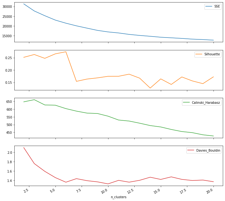
df_cluster_scorer.plot.line(subplots=True,x ='n_clusters', figsize=(12,12))
array([<AxesSubplot:xlabel='n_clusters'>,
       <AxesSubplot:xlabel='n_clusters'>,
       <AxesSubplot:xlabel='n_clusters'>,
       <AxesSubplot:xlabel='n_clusters'>], dtype=object)
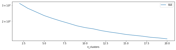
df_cluster_scorer.plot.line(y='SSE',x ='n_clusters',logy=True, figsize=(12,3))
<AxesSubplot:xlabel='n_clusters'>
Visualize the cluster
pca = PCA(n_components=2, whiten=True)

pca.fit(city_groups_std[num_list])
PCA(n_components=2, whiten=True)
pca.fit_transform(city_groups_std[num_list])
array([[ 0.09362892, -0.52372539],
       [ 0.84601865, -0.14918922],
       [ 3.82881756, -0.1731645 ],
       ...,
       [ 0.46338984,  1.53211431],
       [-0.97116177, -0.50927138],
       [ 1.16965175,  1.06541916]])
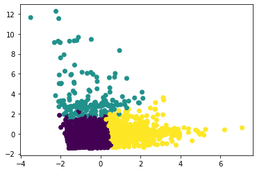
city_groups_std['x'], city_groups_std['y'] = zip(*(pca.fit_transform(city_groups_std[num_list])))
plt.scatter(city_groups_std['x'], city_groups_std['y'], c=city_groups_std['cluster'])
plt.show()
df_cluster_scorer[df_cluster_scorer['n_clusters']==2]['model'].values[0]
KMeans(n_clusters=2)
@interact
def show_clusters(n=(2,20)):
    model = df_cluster_scorer[df_cluster_scorer['n_clusters']==n]['model'].values[0]
    labels = model.predict(city_groups_std[num_list])
    plt.scatter(city_groups_std['x'], city_groups_std['y'], c=labels)
    plt.title(f"Cluster {n}")
    plt.show()
Step4. Profile the cluster
city_groups.merge(city_groups_std[['user_location_city', 'cluster']]).groupby('cluster').mean()
| user_location_city | orig_destination_distance | is_mobile | is_package | srch_adults_cnt | srch_children_cnt | srch_rm_cnt | duration | days_in_advance | |
|---|---|---|---|---|---|---|---|---|---|
| cluster | |||||||||
| 0 | 28059.919851 | 1390.514992 | 0.137752 | 0.184819 | 1.994703 | 0.377777 | 1.069875 | 2.794248 | 42.493643 |
| 1 | 31017.981928 | 1525.042593 | 0.115663 | 0.196687 | 4.084940 | 0.567671 | 2.412249 | 3.069378 | 55.478239 |
| 2 | 28893.937273 | 3189.285509 | 0.112741 | 0.487444 | 2.029138 | 0.321586 | 1.069821 | 5.300009 | 101.977415 |
Step 5: assess the statistical robustness
A statistically robust segmentation return similar results using different clustering methodologies