Cohort Analysis using Online Retail Dataset from UCI

Imports
from fastai.basics import *
from nlphero.data.external import *
import sklearn as sk
import bqplot as bq
import seaborn as sns
import datetime as dt
import statsmodels.api as sm
from sklearn.preprocessing import StandardScaler, FunctionTransformer
from sklearn.decomposition import PCA

from sklearn import metrics
from sklearn.cluster import KMeans
from scipy import stats
from ipywidgets import interact, interactive

import warnings
%matplotlib inline

warnings.filterwarnings("ignore")
Read the Data
# kaggle datasets download -d jihyeseo/online-retail-data-set-from-uci-ml-repo
path = untar_data("kaggle_datasets::jihyeseo/online-retail-data-set-from-uci-ml-repo"); path
Path('/Landmark2/pdo/.nlphero/data/online-retail-data-set-from-uci-ml-repo')
path.ls()
(#1) [Path('/Landmark2/pdo/.nlphero/data/online-retail-data-set-from-uci-ml-repo/Online Retail.xlsx')]
df = pd.read_excel(path/"Online Retail.xlsx", parse_dates=['InvoiceDate'])
df.head()
| InvoiceNo | StockCode | Description | Quantity | InvoiceDate | UnitPrice | CustomerID | Country | |
|---|---|---|---|---|---|---|---|---|
| 0 | 536365 | 85123A | WHITE HANGING HEART T-LIGHT HOLDER | 6 | 2010-12-01 08:26:00 | 2.55 | 17850.0 | United Kingdom |
| 1 | 536365 | 71053 | WHITE METAL LANTERN | 6 | 2010-12-01 08:26:00 | 3.39 | 17850.0 | United Kingdom |
| 2 | 536365 | 84406B | CREAM CUPID HEARTS COAT HANGER | 8 | 2010-12-01 08:26:00 | 2.75 | 17850.0 | United Kingdom |
| 3 | 536365 | 84029G | KNITTED UNION FLAG HOT WATER BOTTLE | 6 | 2010-12-01 08:26:00 | 3.39 | 17850.0 | United Kingdom |
| 4 | 536365 | 84029E | RED WOOLLY HOTTIE WHITE HEART. | 6 | 2010-12-01 08:26:00 | 3.39 | 17850.0 | United Kingdom |
df.info()
<class 'pandas.core.frame.DataFrame'>
RangeIndex: 541909 entries, 0 to 541908
Data columns (total 8 columns):
 #   Column       Non-Null Count   Dtype
---  ------       --------------   -----
 0   InvoiceNo    541909 non-null  object
 1   StockCode    541909 non-null  object
 2   Description  540455 non-null  object
 3   Quantity     541909 non-null  int64
 4   InvoiceDate  541909 non-null  datetime64[ns]
 5   UnitPrice    541909 non-null  float64
 6   CustomerID   406829 non-null  float64
 7   Country      541909 non-null  object
dtypes: datetime64[ns](1), float64(2), int64(1), object(4)
memory usage: 33.1+ MB
df.describe()
| Quantity | UnitPrice | CustomerID | |
|---|---|---|---|
| count | 541909.000000 | 541909.000000 | 406829.000000 |
| mean | 9.552250 | 4.611114 | 15287.690570 |
| std | 218.081158 | 96.759853 | 1713.600303 |
| min | -80995.000000 | -11062.060000 | 12346.000000 |
| 25% | 1.000000 | 1.250000 | 13953.000000 |
| 50% | 3.000000 | 2.080000 | 15152.000000 |
| 75% | 10.000000 | 4.130000 | 16791.000000 |
| max | 80995.000000 | 38970.000000 | 18287.000000 |
df.nunique()
InvoiceNo      25900
StockCode       4070
Description     4223
Quantity         722
InvoiceDate    23260
UnitPrice       1630
CustomerID      4372
Country           38
dtype: int64
Data Cleaning
df.isnull().sum()
InvoiceNo           0
StockCode           0
Description      1454
Quantity            0
InvoiceDate         0
UnitPrice           0
CustomerID     135080
Country             0
dtype: int64
df[df.duplicated()]
| InvoiceNo | StockCode | Description | Quantity | InvoiceDate | UnitPrice | CustomerID | Country | |
|---|---|---|---|---|---|---|---|---|
| 517 | 536409 | 21866 | UNION JACK FLAG LUGGAGE TAG | 1 | 2010-12-01 11:45:00 | 1.25 | 17908.0 | United Kingdom |
| 527 | 536409 | 22866 | HAND WARMER SCOTTY DOG DESIGN | 1 | 2010-12-01 11:45:00 | 2.10 | 17908.0 | United Kingdom |
| 537 | 536409 | 22900 | SET 2 TEA TOWELS I LOVE LONDON | 1 | 2010-12-01 11:45:00 | 2.95 | 17908.0 | United Kingdom |
| 539 | 536409 | 22111 | SCOTTIE DOG HOT WATER BOTTLE | 1 | 2010-12-01 11:45:00 | 4.95 | 17908.0 | United Kingdom |
| 555 | 536412 | 22327 | ROUND SNACK BOXES SET OF 4 SKULLS | 1 | 2010-12-01 11:49:00 | 2.95 | 17920.0 | United Kingdom |
| ... | ... | ... | ... | ... | ... | ... | ... | ... |
| 541675 | 581538 | 22068 | BLACK PIRATE TREASURE CHEST | 1 | 2011-12-09 11:34:00 | 0.39 | 14446.0 | United Kingdom |
| 541689 | 581538 | 23318 | BOX OF 6 MINI VINTAGE CRACKERS | 1 | 2011-12-09 11:34:00 | 2.49 | 14446.0 | United Kingdom |
| 541692 | 581538 | 22992 | REVOLVER WOODEN RULER | 1 | 2011-12-09 11:34:00 | 1.95 | 14446.0 | United Kingdom |
| 541699 | 581538 | 22694 | WICKER STAR | 1 | 2011-12-09 11:34:00 | 2.10 | 14446.0 | United Kingdom |
| 541701 | 581538 | 23343 | JUMBO BAG VINTAGE CHRISTMAS | 1 | 2011-12-09 11:34:00 | 2.08 | 14446.0 | United Kingdom |
5268 rows × 8 columns
Remove null and duplicates
df =df[~df.isnull()];
df
| InvoiceNo | StockCode | Description | Quantity | InvoiceDate | UnitPrice | CustomerID | Country | |
|---|---|---|---|---|---|---|---|---|
| 0 | 536365 | 85123A | WHITE HANGING HEART T-LIGHT HOLDER | 6 | 2010-12-01 08:26:00 | 2.55 | 17850.0 | United Kingdom |
| 1 | 536365 | 71053 | WHITE METAL LANTERN | 6 | 2010-12-01 08:26:00 | 3.39 | 17850.0 | United Kingdom |
| 2 | 536365 | 84406B | CREAM CUPID HEARTS COAT HANGER | 8 | 2010-12-01 08:26:00 | 2.75 | 17850.0 | United Kingdom |
| 3 | 536365 | 84029G | KNITTED UNION FLAG HOT WATER BOTTLE | 6 | 2010-12-01 08:26:00 | 3.39 | 17850.0 | United Kingdom |
| 4 | 536365 | 84029E | RED WOOLLY HOTTIE WHITE HEART. | 6 | 2010-12-01 08:26:00 | 3.39 | 17850.0 | United Kingdom |
| ... | ... | ... | ... | ... | ... | ... | ... | ... |
| 541904 | 581587 | 22613 | PACK OF 20 SPACEBOY NAPKINS | 12 | 2011-12-09 12:50:00 | 0.85 | 12680.0 | France |
| 541905 | 581587 | 22899 | CHILDREN'S APRON DOLLY GIRL | 6 | 2011-12-09 12:50:00 | 2.10 | 12680.0 | France |
| 541906 | 581587 | 23254 | CHILDRENS CUTLERY DOLLY GIRL | 4 | 2011-12-09 12:50:00 | 4.15 | 12680.0 | France |
| 541907 | 581587 | 23255 | CHILDRENS CUTLERY CIRCUS PARADE | 4 | 2011-12-09 12:50:00 | 4.15 | 12680.0 | France |
| 541908 | 581587 | 22138 | BAKING SET 9 PIECE RETROSPOT | 3 | 2011-12-09 12:50:00 | 4.95 | 12680.0 | France |
541909 rows × 8 columns
# df = df[~df.duplicated()]
df = df.drop_duplicates();
df
| InvoiceNo | StockCode | Description | Quantity | InvoiceDate | UnitPrice | CustomerID | Country | |
|---|---|---|---|---|---|---|---|---|
| 0 | 536365 | 85123A | WHITE HANGING HEART T-LIGHT HOLDER | 6 | 2010-12-01 08:26:00 | 2.55 | 17850.0 | United Kingdom |
| 1 | 536365 | 71053 | WHITE METAL LANTERN | 6 | 2010-12-01 08:26:00 | 3.39 | 17850.0 | United Kingdom |
| 2 | 536365 | 84406B | CREAM CUPID HEARTS COAT HANGER | 8 | 2010-12-01 08:26:00 | 2.75 | 17850.0 | United Kingdom |
| 3 | 536365 | 84029G | KNITTED UNION FLAG HOT WATER BOTTLE | 6 | 2010-12-01 08:26:00 | 3.39 | 17850.0 | United Kingdom |
| 4 | 536365 | 84029E | RED WOOLLY HOTTIE WHITE HEART. | 6 | 2010-12-01 08:26:00 | 3.39 | 17850.0 | United Kingdom |
| ... | ... | ... | ... | ... | ... | ... | ... | ... |
| 541904 | 581587 | 22613 | PACK OF 20 SPACEBOY NAPKINS | 12 | 2011-12-09 12:50:00 | 0.85 | 12680.0 | France |
| 541905 | 581587 | 22899 | CHILDREN'S APRON DOLLY GIRL | 6 | 2011-12-09 12:50:00 | 2.10 | 12680.0 | France |
| 541906 | 581587 | 23254 | CHILDRENS CUTLERY DOLLY GIRL | 4 | 2011-12-09 12:50:00 | 4.15 | 12680.0 | France |
| 541907 | 581587 | 23255 | CHILDRENS CUTLERY CIRCUS PARADE | 4 | 2011-12-09 12:50:00 | 4.15 | 12680.0 | France |
| 541908 | 581587 | 22138 | BAKING SET 9 PIECE RETROSPOT | 3 | 2011-12-09 12:50:00 | 4.95 | 12680.0 | France |
536641 rows × 8 columns
df[df.isnull()].sum()
InvoiceNo      0.0
StockCode      0.0
Description    0.0
Quantity       0.0
UnitPrice      0.0
CustomerID     0.0
Country        0.0
dtype: float64
df[df.duplicated()]
| InvoiceNo | StockCode | Description | Quantity | InvoiceDate | UnitPrice | CustomerID | Country |
|---|
df.loc[:,'CustomerID'] = df['CustomerID'].astype('category').values
df.describe()
| Quantity | UnitPrice | CohortIndex | TotalSum | |
|---|---|---|---|---|
| count | 524878.000000 | 524878.000000 | 392692.000000 | 524878.000000 |
| mean | 10.616600 | 3.922573 | 5.147599 | 20.275399 |
| std | 156.280031 | 36.093028 | 3.850198 | 271.693566 |
| min | 1.000000 | 0.001000 | 1.000000 | 0.001000 |
| 25% | 1.000000 | 1.250000 | 1.000000 | 3.900000 |
| 50% | 4.000000 | 2.080000 | 4.000000 | 9.920000 |
| 75% | 11.000000 | 4.130000 | 8.000000 | 17.700000 |
| max | 80995.000000 | 13541.330000 | 13.000000 | 168469.600000 |
Warning
Some negative values for minimum, need to remove more rows.
Remove Negative Quantities and Unit Price
df[df['Quantity']<0]
| InvoiceNo | StockCode | Description | Quantity | InvoiceDate | UnitPrice | CustomerID | Country | |
|---|---|---|---|---|---|---|---|---|
| 141 | C536379 | D | Discount | -1 | 2010-12-01 09:41:00 | 27.50 | 14527.0 | United Kingdom |
| 154 | C536383 | 35004C | SET OF 3 COLOURED FLYING DUCKS | -1 | 2010-12-01 09:49:00 | 4.65 | 15311.0 | United Kingdom |
| 235 | C536391 | 22556 | PLASTERS IN TIN CIRCUS PARADE | -12 | 2010-12-01 10:24:00 | 1.65 | 17548.0 | United Kingdom |
| 236 | C536391 | 21984 | PACK OF 12 PINK PAISLEY TISSUES | -24 | 2010-12-01 10:24:00 | 0.29 | 17548.0 | United Kingdom |
| 237 | C536391 | 21983 | PACK OF 12 BLUE PAISLEY TISSUES | -24 | 2010-12-01 10:24:00 | 0.29 | 17548.0 | United Kingdom |
| ... | ... | ... | ... | ... | ... | ... | ... | ... |
| 540449 | C581490 | 23144 | ZINC T-LIGHT HOLDER STARS SMALL | -11 | 2011-12-09 09:57:00 | 0.83 | 14397.0 | United Kingdom |
| 541541 | C581499 | M | Manual | -1 | 2011-12-09 10:28:00 | 224.69 | 15498.0 | United Kingdom |
| 541715 | C581568 | 21258 | VICTORIAN SEWING BOX LARGE | -5 | 2011-12-09 11:57:00 | 10.95 | 15311.0 | United Kingdom |
| 541716 | C581569 | 84978 | HANGING HEART JAR T-LIGHT HOLDER | -1 | 2011-12-09 11:58:00 | 1.25 | 17315.0 | United Kingdom |
| 541717 | C581569 | 20979 | 36 PENCILS TUBE RED RETROSPOT | -5 | 2011-12-09 11:58:00 | 1.25 | 17315.0 | United Kingdom |
10587 rows × 8 columns
df[df['UnitPrice']<0]
| InvoiceNo | StockCode | Description | Quantity | InvoiceDate | UnitPrice | CustomerID | Country | |
|---|---|---|---|---|---|---|---|---|
| 299983 | A563186 | B | Adjust bad debt | 1 | 2011-08-12 14:51:00 | -11062.06 | NaN | United Kingdom |
| 299984 | A563187 | B | Adjust bad debt | 1 | 2011-08-12 14:52:00 | -11062.06 | NaN | United Kingdom |
df[(df['Quantity']>0)&(df['UnitPrice']>0)]
| InvoiceNo | StockCode | Description | Quantity | InvoiceDate | UnitPrice | CustomerID | Country | |
|---|---|---|---|---|---|---|---|---|
| 0 | 536365 | 85123A | WHITE HANGING HEART T-LIGHT HOLDER | 6 | 2010-12-01 08:26:00 | 2.55 | 17850.0 | United Kingdom |
| 1 | 536365 | 71053 | WHITE METAL LANTERN | 6 | 2010-12-01 08:26:00 | 3.39 | 17850.0 | United Kingdom |
| 2 | 536365 | 84406B | CREAM CUPID HEARTS COAT HANGER | 8 | 2010-12-01 08:26:00 | 2.75 | 17850.0 | United Kingdom |
| 3 | 536365 | 84029G | KNITTED UNION FLAG HOT WATER BOTTLE | 6 | 2010-12-01 08:26:00 | 3.39 | 17850.0 | United Kingdom |
| 4 | 536365 | 84029E | RED WOOLLY HOTTIE WHITE HEART. | 6 | 2010-12-01 08:26:00 | 3.39 | 17850.0 | United Kingdom |
| ... | ... | ... | ... | ... | ... | ... | ... | ... |
| 541904 | 581587 | 22613 | PACK OF 20 SPACEBOY NAPKINS | 12 | 2011-12-09 12:50:00 | 0.85 | 12680.0 | France |
| 541905 | 581587 | 22899 | CHILDREN'S APRON DOLLY GIRL | 6 | 2011-12-09 12:50:00 | 2.10 | 12680.0 | France |
| 541906 | 581587 | 23254 | CHILDRENS CUTLERY DOLLY GIRL | 4 | 2011-12-09 12:50:00 | 4.15 | 12680.0 | France |
| 541907 | 581587 | 23255 | CHILDRENS CUTLERY CIRCUS PARADE | 4 | 2011-12-09 12:50:00 | 4.15 | 12680.0 | France |
| 541908 | 581587 | 22138 | BAKING SET 9 PIECE RETROSPOT | 3 | 2011-12-09 12:50:00 | 4.95 | 12680.0 | France |
524878 rows × 8 columns
df = df[(df['Quantity']>0)&(df['UnitPrice']>0)]; df.describe()
| Quantity | UnitPrice | |
|---|---|---|
| count | 524878.000000 | 524878.000000 |
| mean | 10.616600 | 3.922573 |
| std | 156.280031 | 36.093028 |
| min | 1.000000 | 0.001000 |
| 25% | 1.000000 | 1.250000 |
| 50% | 4.000000 | 2.080000 |
| 75% | 11.000000 | 4.130000 |
| max | 80995.000000 | 13541.330000 |
df.shape
(524878, 8)
df.groupby('CustomerID').count()
| InvoiceNo | StockCode | Description | Quantity | InvoiceDate | UnitPrice | Country | |
|---|---|---|---|---|---|---|---|
| CustomerID | |||||||
| 12346.0 | 1 | 1 | 1 | 1 | 1 | 1 | 1 |
| 12347.0 | 182 | 182 | 182 | 182 | 182 | 182 | 182 |
| 12348.0 | 31 | 31 | 31 | 31 | 31 | 31 | 31 |
| 12349.0 | 73 | 73 | 73 | 73 | 73 | 73 | 73 |
| 12350.0 | 17 | 17 | 17 | 17 | 17 | 17 | 17 |
| ... | ... | ... | ... | ... | ... | ... | ... |
| 18280.0 | 10 | 10 | 10 | 10 | 10 | 10 | 10 |
| 18281.0 | 7 | 7 | 7 | 7 | 7 | 7 | 7 |
| 18282.0 | 12 | 12 | 12 | 12 | 12 | 12 | 12 |
| 18283.0 | 721 | 721 | 721 | 721 | 721 | 721 | 721 |
| 18287.0 | 70 | 70 | 70 | 70 | 70 | 70 | 70 |
4372 rows × 7 columns
# df.groupby(['CustomerID', 'InvoiceNo']).count()
df.nunique()
InvoiceNo      19960
StockCode       3922
Description     4026
Quantity         375
InvoiceDate    18499
UnitPrice       1291
CustomerID      4338
Country           38
dtype: int64
df[df['CustomerID']==12347.0]
| InvoiceNo | StockCode | Description | Quantity | InvoiceDate | UnitPrice | CustomerID | Country | |
|---|---|---|---|---|---|---|---|---|
| 14938 | 537626 | 85116 | BLACK CANDELABRA T-LIGHT HOLDER | 12 | 2010-12-07 14:57:00 | 2.10 | 12347.0 | Iceland |
| 14939 | 537626 | 22375 | AIRLINE BAG VINTAGE JET SET BROWN | 4 | 2010-12-07 14:57:00 | 4.25 | 12347.0 | Iceland |
| 14940 | 537626 | 71477 | COLOUR GLASS. STAR T-LIGHT HOLDER | 12 | 2010-12-07 14:57:00 | 3.25 | 12347.0 | Iceland |
| 14941 | 537626 | 22492 | MINI PAINT SET VINTAGE | 36 | 2010-12-07 14:57:00 | 0.65 | 12347.0 | Iceland |
| 14942 | 537626 | 22771 | CLEAR DRAWER KNOB ACRYLIC EDWARDIAN | 12 | 2010-12-07 14:57:00 | 1.25 | 12347.0 | Iceland |
| ... | ... | ... | ... | ... | ... | ... | ... | ... |
| 535010 | 581180 | 20719 | WOODLAND CHARLOTTE BAG | 10 | 2011-12-07 15:52:00 | 0.85 | 12347.0 | Iceland |
| 535011 | 581180 | 21265 | PINK GOOSE FEATHER TREE 60CM | 12 | 2011-12-07 15:52:00 | 1.95 | 12347.0 | Iceland |
| 535012 | 581180 | 23271 | CHRISTMAS TABLE SILVER CANDLE SPIKE | 16 | 2011-12-07 15:52:00 | 0.83 | 12347.0 | Iceland |
| 535013 | 581180 | 23506 | MINI PLAYING CARDS SPACEBOY | 20 | 2011-12-07 15:52:00 | 0.42 | 12347.0 | Iceland |
| 535014 | 581180 | 23508 | MINI PLAYING CARDS DOLLY GIRL | 20 | 2011-12-07 15:52:00 | 0.42 | 12347.0 | Iceland |
182 rows × 8 columns
Cohort Analysis
Note
Group of subjects sharing defining characteristics
Observe across time
Compare with other cohorts
Areas to perform a cross-section(compare difference across subjects) at interval through time
Type of cohorts
Time Cohorts
Customer who signed up for a product or service during a particular time frame.
Analysis -> Customer behaviour at time of purchase[ monthly, quaterly or daily]
Behaviour Cohorts
Customer who purchased a kind of product or subscribed to a behaviour
Understanding needs [ Basic or Advanced based on signup]
Custom Made services for a particular segment
Size Cohorts
Various sizes of customers who purchase products or services
Amount of spending in some periodic time afer acquisition
Product type that customer most of their order amount in some period of time.
Making Cohort Analysis
We need to create labels
Invoice period - Year & month of a single transaction
Cohort group - Year & month of customer first purchase
Cohort period/ Cohort index - Customer stage in its lifetime(int). It is number of months passed since first purchase
Code Construction on Sample
sample = df[df['CustomerID'].isin([12347.0, 18283.0, 18287.0])].reset_index(drop=True); sample
| InvoiceNo | StockCode | Description | Quantity | InvoiceDate | UnitPrice | CustomerID | Country | |
|---|---|---|---|---|---|---|---|---|
| 0 | 537626 | 85116 | BLACK CANDELABRA T-LIGHT HOLDER | 12 | 2010-12-07 14:57:00 | 2.10 | 12347.0 | Iceland |
| 1 | 537626 | 22375 | AIRLINE BAG VINTAGE JET SET BROWN | 4 | 2010-12-07 14:57:00 | 4.25 | 12347.0 | Iceland |
| 2 | 537626 | 71477 | COLOUR GLASS. STAR T-LIGHT HOLDER | 12 | 2010-12-07 14:57:00 | 3.25 | 12347.0 | Iceland |
| 3 | 537626 | 22492 | MINI PAINT SET VINTAGE | 36 | 2010-12-07 14:57:00 | 0.65 | 12347.0 | Iceland |
| 4 | 537626 | 22771 | CLEAR DRAWER KNOB ACRYLIC EDWARDIAN | 12 | 2010-12-07 14:57:00 | 1.25 | 12347.0 | Iceland |
| ... | ... | ... | ... | ... | ... | ... | ... | ... |
| 968 | 581180 | 20719 | WOODLAND CHARLOTTE BAG | 10 | 2011-12-07 15:52:00 | 0.85 | 12347.0 | Iceland |
| 969 | 581180 | 21265 | PINK GOOSE FEATHER TREE 60CM | 12 | 2011-12-07 15:52:00 | 1.95 | 12347.0 | Iceland |
| 970 | 581180 | 23271 | CHRISTMAS TABLE SILVER CANDLE SPIKE | 16 | 2011-12-07 15:52:00 | 0.83 | 12347.0 | Iceland |
| 971 | 581180 | 23506 | MINI PLAYING CARDS SPACEBOY | 20 | 2011-12-07 15:52:00 | 0.42 | 12347.0 | Iceland |
| 972 | 581180 | 23508 | MINI PLAYING CARDS DOLLY GIRL | 20 | 2011-12-07 15:52:00 | 0.42 | 12347.0 | Iceland |
973 rows × 8 columns
# sample['InvoiceDate'][0]
x = sample['InvoiceDate'][0]

x.year, x.month, dt.datetime(x.year, x.month, 1)
# x
(2010, 12, datetime.datetime(2010, 12, 1, 0, 0))
sample['InvoiceMonth'] = sample['InvoiceDate']\
.apply(lambda x : dt.datetime(x.year, x.month, 1))

sample
| InvoiceNo | StockCode | Description | Quantity | InvoiceDate | UnitPrice | CustomerID | Country | InvoiceMonth | |
|---|---|---|---|---|---|---|---|---|---|
| 0 | 537626 | 85116 | BLACK CANDELABRA T-LIGHT HOLDER | 12 | 2010-12-07 14:57:00 | 2.10 | 12347.0 | Iceland | 2010-12-01 |
| 1 | 537626 | 22375 | AIRLINE BAG VINTAGE JET SET BROWN | 4 | 2010-12-07 14:57:00 | 4.25 | 12347.0 | Iceland | 2010-12-01 |
| 2 | 537626 | 71477 | COLOUR GLASS. STAR T-LIGHT HOLDER | 12 | 2010-12-07 14:57:00 | 3.25 | 12347.0 | Iceland | 2010-12-01 |
| 3 | 537626 | 22492 | MINI PAINT SET VINTAGE | 36 | 2010-12-07 14:57:00 | 0.65 | 12347.0 | Iceland | 2010-12-01 |
| 4 | 537626 | 22771 | CLEAR DRAWER KNOB ACRYLIC EDWARDIAN | 12 | 2010-12-07 14:57:00 | 1.25 | 12347.0 | Iceland | 2010-12-01 |
| ... | ... | ... | ... | ... | ... | ... | ... | ... | ... |
| 968 | 581180 | 20719 | WOODLAND CHARLOTTE BAG | 10 | 2011-12-07 15:52:00 | 0.85 | 12347.0 | Iceland | 2011-12-01 |
| 969 | 581180 | 21265 | PINK GOOSE FEATHER TREE 60CM | 12 | 2011-12-07 15:52:00 | 1.95 | 12347.0 | Iceland | 2011-12-01 |
| 970 | 581180 | 23271 | CHRISTMAS TABLE SILVER CANDLE SPIKE | 16 | 2011-12-07 15:52:00 | 0.83 | 12347.0 | Iceland | 2011-12-01 |
| 971 | 581180 | 23506 | MINI PLAYING CARDS SPACEBOY | 20 | 2011-12-07 15:52:00 | 0.42 | 12347.0 | Iceland | 2011-12-01 |
| 972 | 581180 | 23508 | MINI PLAYING CARDS DOLLY GIRL | 20 | 2011-12-07 15:52:00 | 0.42 | 12347.0 | Iceland | 2011-12-01 |
973 rows × 9 columns
sample.groupby('CustomerID')['InvoiceMonth'].transform('min')
0     2010-12-01
1     2010-12-01
2     2010-12-01
3     2010-12-01
4     2010-12-01
         ...
968   2010-12-01
969   2010-12-01
970   2010-12-01
971   2010-12-01
972   2010-12-01
Name: InvoiceMonth, Length: 973, dtype: datetime64[ns]
sample['CohortMonth']= sample.groupby('CustomerID')['InvoiceMonth'].transform('min')
sample
| InvoiceNo | StockCode | Description | Quantity | InvoiceDate | UnitPrice | CustomerID | Country | InvoiceMonth | CohortMonth | |
|---|---|---|---|---|---|---|---|---|---|---|
| 0 | 537626 | 85116 | BLACK CANDELABRA T-LIGHT HOLDER | 12 | 2010-12-07 14:57:00 | 2.10 | 12347.0 | Iceland | 2010-12-01 | 2010-12-01 |
| 1 | 537626 | 22375 | AIRLINE BAG VINTAGE JET SET BROWN | 4 | 2010-12-07 14:57:00 | 4.25 | 12347.0 | Iceland | 2010-12-01 | 2010-12-01 |
| 2 | 537626 | 71477 | COLOUR GLASS. STAR T-LIGHT HOLDER | 12 | 2010-12-07 14:57:00 | 3.25 | 12347.0 | Iceland | 2010-12-01 | 2010-12-01 |
| 3 | 537626 | 22492 | MINI PAINT SET VINTAGE | 36 | 2010-12-07 14:57:00 | 0.65 | 12347.0 | Iceland | 2010-12-01 | 2010-12-01 |
| 4 | 537626 | 22771 | CLEAR DRAWER KNOB ACRYLIC EDWARDIAN | 12 | 2010-12-07 14:57:00 | 1.25 | 12347.0 | Iceland | 2010-12-01 | 2010-12-01 |
| ... | ... | ... | ... | ... | ... | ... | ... | ... | ... | ... |
| 968 | 581180 | 20719 | WOODLAND CHARLOTTE BAG | 10 | 2011-12-07 15:52:00 | 0.85 | 12347.0 | Iceland | 2011-12-01 | 2010-12-01 |
| 969 | 581180 | 21265 | PINK GOOSE FEATHER TREE 60CM | 12 | 2011-12-07 15:52:00 | 1.95 | 12347.0 | Iceland | 2011-12-01 | 2010-12-01 |
| 970 | 581180 | 23271 | CHRISTMAS TABLE SILVER CANDLE SPIKE | 16 | 2011-12-07 15:52:00 | 0.83 | 12347.0 | Iceland | 2011-12-01 | 2010-12-01 |
| 971 | 581180 | 23506 | MINI PLAYING CARDS SPACEBOY | 20 | 2011-12-07 15:52:00 | 0.42 | 12347.0 | Iceland | 2011-12-01 | 2010-12-01 |
| 972 | 581180 | 23508 | MINI PLAYING CARDS DOLLY GIRL | 20 | 2011-12-07 15:52:00 | 0.42 | 12347.0 | Iceland | 2011-12-01 | 2010-12-01 |
973 rows × 10 columns
((sample['InvoiceMonth'] - sample['CohortMonth'])/(np.timedelta64(1, 'M'))).astype(int)
0       0
1       0
2       0
3       0
4       0
       ..
968    11
969    11
970    11
971    11
972    11
Length: 973, dtype: int64
def get_month_int (dframe,column):
    year = dframe[column].dt.year
    month = dframe[column].dt.month
    day = dframe[column].dt.day
    return year, month , day

invoice_year,invoice_month,_ = get_month_int(sample,'InvoiceMonth')
cohort_year,cohort_month,_ = get_month_int(sample,'CohortMonth')

year_diff = invoice_year - cohort_year
month_diff = invoice_month - cohort_month

year_diff * 12 + month_diff + 1 # , year_diff, month_diff
0       1
1       1
2       1
3       1
4       1
       ..
968    13
969    13
970    13
971    13
972    13
Length: 973, dtype: int64
(sample['InvoiceMonth'].dt.year - sample['CohortMonth'].dt.year)*12\
+(sample['InvoiceMonth'].dt.month - sample['CohortMonth'].dt.month)\
+1
0       1
1       1
2       1
3       1
4       1
       ..
968    13
969    13
970    13
971    13
972    13
Length: 973, dtype: int64
sample['CohortIndex'] = (sample['InvoiceMonth'].dt.year - sample['CohortMonth'].dt.year)*12\
+(sample['InvoiceMonth'].dt.month - sample['CohortMonth'].dt.month)\
+1

sample
| InvoiceNo | StockCode | Description | Quantity | InvoiceDate | UnitPrice | CustomerID | Country | InvoiceMonth | CohortMonth | CohortIndex | |
|---|---|---|---|---|---|---|---|---|---|---|---|
| 0 | 537626 | 85116 | BLACK CANDELABRA T-LIGHT HOLDER | 12 | 2010-12-07 14:57:00 | 2.10 | 12347.0 | Iceland | 2010-12-01 | 2010-12-01 | 1 |
| 1 | 537626 | 22375 | AIRLINE BAG VINTAGE JET SET BROWN | 4 | 2010-12-07 14:57:00 | 4.25 | 12347.0 | Iceland | 2010-12-01 | 2010-12-01 | 1 |
| 2 | 537626 | 71477 | COLOUR GLASS. STAR T-LIGHT HOLDER | 12 | 2010-12-07 14:57:00 | 3.25 | 12347.0 | Iceland | 2010-12-01 | 2010-12-01 | 1 |
| 3 | 537626 | 22492 | MINI PAINT SET VINTAGE | 36 | 2010-12-07 14:57:00 | 0.65 | 12347.0 | Iceland | 2010-12-01 | 2010-12-01 | 1 |
| 4 | 537626 | 22771 | CLEAR DRAWER KNOB ACRYLIC EDWARDIAN | 12 | 2010-12-07 14:57:00 | 1.25 | 12347.0 | Iceland | 2010-12-01 | 2010-12-01 | 1 |
| ... | ... | ... | ... | ... | ... | ... | ... | ... | ... | ... | ... |
| 968 | 581180 | 20719 | WOODLAND CHARLOTTE BAG | 10 | 2011-12-07 15:52:00 | 0.85 | 12347.0 | Iceland | 2011-12-01 | 2010-12-01 | 13 |
| 969 | 581180 | 21265 | PINK GOOSE FEATHER TREE 60CM | 12 | 2011-12-07 15:52:00 | 1.95 | 12347.0 | Iceland | 2011-12-01 | 2010-12-01 | 13 |
| 970 | 581180 | 23271 | CHRISTMAS TABLE SILVER CANDLE SPIKE | 16 | 2011-12-07 15:52:00 | 0.83 | 12347.0 | Iceland | 2011-12-01 | 2010-12-01 | 13 |
| 971 | 581180 | 23506 | MINI PLAYING CARDS SPACEBOY | 20 | 2011-12-07 15:52:00 | 0.42 | 12347.0 | Iceland | 2011-12-01 | 2010-12-01 | 13 |
| 972 | 581180 | 23508 | MINI PLAYING CARDS DOLLY GIRL | 20 | 2011-12-07 15:52:00 | 0.42 | 12347.0 | Iceland | 2011-12-01 | 2010-12-01 | 13 |
973 rows × 11 columns
sample_data = sample.groupby(['CohortMonth', 'CohortIndex'])['CustomerID'].apply(pd.Series.nunique).reset_index()
sample_data
| CohortMonth | CohortIndex | CustomerID | |
|---|---|---|---|
| 0 | 2010-12-01 | 1 | 1 |
| 1 | 2010-12-01 | 2 | 1 |
| 2 | 2010-12-01 | 5 | 1 |
| 3 | 2010-12-01 | 7 | 1 |
| 4 | 2010-12-01 | 9 | 1 |
| 5 | 2010-12-01 | 11 | 1 |
| 6 | 2010-12-01 | 13 | 1 |
| 7 | 2011-01-01 | 1 | 1 |
| 8 | 2011-01-01 | 2 | 1 |
| 9 | 2011-01-01 | 4 | 1 |
| 10 | 2011-01-01 | 5 | 1 |
| 11 | 2011-01-01 | 6 | 1 |
| 12 | 2011-01-01 | 7 | 1 |
| 13 | 2011-01-01 | 9 | 1 |
| 14 | 2011-01-01 | 10 | 1 |
| 15 | 2011-01-01 | 11 | 1 |
| 16 | 2011-01-01 | 12 | 1 |
| 17 | 2011-05-01 | 1 | 1 |
| 18 | 2011-05-01 | 6 | 1 |
sample_data.pivot(index='CohortMonth',
                  columns='CohortIndex',
                  values='CustomerID')
| CohortIndex | 1 | 2 | 4 | 5 | 6 | 7 | 9 | 10 | 11 | 12 | 13 |
|---|---|---|---|---|---|---|---|---|---|---|---|
| CohortMonth | |||||||||||
| 2010-12-01 | 1.0 | 1.0 | NaN | 1.0 | NaN | 1.0 | 1.0 | NaN | 1.0 | NaN | 1.0 |
| 2011-01-01 | 1.0 | 1.0 | 1.0 | 1.0 | 1.0 | 1.0 | 1.0 | 1.0 | 1.0 | 1.0 | NaN |
| 2011-05-01 | 1.0 | NaN | NaN | NaN | 1.0 | NaN | NaN | NaN | NaN | NaN | NaN |
Actual Data
InvoiceMonth
df['InvoiceMonth'] = df['InvoiceDate']\
.apply(lambda x : dt.datetime(x.year, x.month, 1))

df
<ipython-input-190-52184b66dd0e>:1: SettingWithCopyWarning:
A value is trying to be set on a copy of a slice from a DataFrame.
Try using .loc[row_indexer,col_indexer] = value instead

See the caveats in the documentation: https://pandas.pydata.org/pandas-docs/stable/user_guide/indexing.html#returning-a-view-versus-a-copy
  df['InvoiceMonth'] = df['InvoiceDate']\
| InvoiceNo | StockCode | Description | Quantity | InvoiceDate | UnitPrice | CustomerID | Country | InvoiceMonth | |
|---|---|---|---|---|---|---|---|---|---|
| 0 | 536365 | 85123A | WHITE HANGING HEART T-LIGHT HOLDER | 6 | 2010-12-01 08:26:00 | 2.55 | 17850.0 | United Kingdom | 2010-12-01 |
| 1 | 536365 | 71053 | WHITE METAL LANTERN | 6 | 2010-12-01 08:26:00 | 3.39 | 17850.0 | United Kingdom | 2010-12-01 |
| 2 | 536365 | 84406B | CREAM CUPID HEARTS COAT HANGER | 8 | 2010-12-01 08:26:00 | 2.75 | 17850.0 | United Kingdom | 2010-12-01 |
| 3 | 536365 | 84029G | KNITTED UNION FLAG HOT WATER BOTTLE | 6 | 2010-12-01 08:26:00 | 3.39 | 17850.0 | United Kingdom | 2010-12-01 |
| 4 | 536365 | 84029E | RED WOOLLY HOTTIE WHITE HEART. | 6 | 2010-12-01 08:26:00 | 3.39 | 17850.0 | United Kingdom | 2010-12-01 |
| ... | ... | ... | ... | ... | ... | ... | ... | ... | ... |
| 541904 | 581587 | 22613 | PACK OF 20 SPACEBOY NAPKINS | 12 | 2011-12-09 12:50:00 | 0.85 | 12680.0 | France | 2011-12-01 |
| 541905 | 581587 | 22899 | CHILDREN'S APRON DOLLY GIRL | 6 | 2011-12-09 12:50:00 | 2.10 | 12680.0 | France | 2011-12-01 |
| 541906 | 581587 | 23254 | CHILDRENS CUTLERY DOLLY GIRL | 4 | 2011-12-09 12:50:00 | 4.15 | 12680.0 | France | 2011-12-01 |
| 541907 | 581587 | 23255 | CHILDRENS CUTLERY CIRCUS PARADE | 4 | 2011-12-09 12:50:00 | 4.15 | 12680.0 | France | 2011-12-01 |
| 541908 | 581587 | 22138 | BAKING SET 9 PIECE RETROSPOT | 3 | 2011-12-09 12:50:00 | 4.95 | 12680.0 | France | 2011-12-01 |
524878 rows × 9 columns
CohortMonth
df['CohortMonth']= df.groupby('CustomerID')['InvoiceMonth'].transform('min'); df
| InvoiceNo | StockCode | Description | Quantity | InvoiceDate | UnitPrice | CustomerID | Country | InvoiceMonth | CohortMonth | CohortIndex | TotalSum | |
|---|---|---|---|---|---|---|---|---|---|---|---|---|
| 0 | 536365 | 85123A | WHITE HANGING HEART T-LIGHT HOLDER | 6 | 2010-12-01 08:26:00 | 2.55 | 17850.0 | United Kingdom | 2010-12-01 | 2010-12-01 | 1.0 | 15.30 |
| 1 | 536365 | 71053 | WHITE METAL LANTERN | 6 | 2010-12-01 08:26:00 | 3.39 | 17850.0 | United Kingdom | 2010-12-01 | 2010-12-01 | 1.0 | 20.34 |
| 2 | 536365 | 84406B | CREAM CUPID HEARTS COAT HANGER | 8 | 2010-12-01 08:26:00 | 2.75 | 17850.0 | United Kingdom | 2010-12-01 | 2010-12-01 | 1.0 | 22.00 |
| 3 | 536365 | 84029G | KNITTED UNION FLAG HOT WATER BOTTLE | 6 | 2010-12-01 08:26:00 | 3.39 | 17850.0 | United Kingdom | 2010-12-01 | 2010-12-01 | 1.0 | 20.34 |
| 4 | 536365 | 84029E | RED WOOLLY HOTTIE WHITE HEART. | 6 | 2010-12-01 08:26:00 | 3.39 | 17850.0 | United Kingdom | 2010-12-01 | 2010-12-01 | 1.0 | 20.34 |
| ... | ... | ... | ... | ... | ... | ... | ... | ... | ... | ... | ... | ... |
| 541904 | 581587 | 22613 | PACK OF 20 SPACEBOY NAPKINS | 12 | 2011-12-09 12:50:00 | 0.85 | 12680.0 | France | 2011-12-01 | 2011-08-01 | 5.0 | 10.20 |
| 541905 | 581587 | 22899 | CHILDREN'S APRON DOLLY GIRL | 6 | 2011-12-09 12:50:00 | 2.10 | 12680.0 | France | 2011-12-01 | 2011-08-01 | 5.0 | 12.60 |
| 541906 | 581587 | 23254 | CHILDRENS CUTLERY DOLLY GIRL | 4 | 2011-12-09 12:50:00 | 4.15 | 12680.0 | France | 2011-12-01 | 2011-08-01 | 5.0 | 16.60 |
| 541907 | 581587 | 23255 | CHILDRENS CUTLERY CIRCUS PARADE | 4 | 2011-12-09 12:50:00 | 4.15 | 12680.0 | France | 2011-12-01 | 2011-08-01 | 5.0 | 16.60 |
| 541908 | 581587 | 22138 | BAKING SET 9 PIECE RETROSPOT | 3 | 2011-12-09 12:50:00 | 4.95 | 12680.0 | France | 2011-12-01 | 2011-08-01 | 5.0 | 14.85 |
524878 rows × 12 columns
CohortIndex
df['CohortIndex'] = (df['InvoiceMonth'].dt.year - df['CohortMonth'].dt.year)*12\
+(df['InvoiceMonth'].dt.month - df['CohortMonth'].dt.month)\
+1

df
| InvoiceNo | StockCode | Description | Quantity | InvoiceDate | UnitPrice | CustomerID | Country | InvoiceMonth | CohortMonth | CohortIndex | TotalSum | |
|---|---|---|---|---|---|---|---|---|---|---|---|---|
| 0 | 536365 | 85123A | WHITE HANGING HEART T-LIGHT HOLDER | 6 | 2010-12-01 08:26:00 | 2.55 | 17850.0 | United Kingdom | 2010-12-01 | 2010-12-01 | 1.0 | 15.30 |
| 1 | 536365 | 71053 | WHITE METAL LANTERN | 6 | 2010-12-01 08:26:00 | 3.39 | 17850.0 | United Kingdom | 2010-12-01 | 2010-12-01 | 1.0 | 20.34 |
| 2 | 536365 | 84406B | CREAM CUPID HEARTS COAT HANGER | 8 | 2010-12-01 08:26:00 | 2.75 | 17850.0 | United Kingdom | 2010-12-01 | 2010-12-01 | 1.0 | 22.00 |
| 3 | 536365 | 84029G | KNITTED UNION FLAG HOT WATER BOTTLE | 6 | 2010-12-01 08:26:00 | 3.39 | 17850.0 | United Kingdom | 2010-12-01 | 2010-12-01 | 1.0 | 20.34 |
| 4 | 536365 | 84029E | RED WOOLLY HOTTIE WHITE HEART. | 6 | 2010-12-01 08:26:00 | 3.39 | 17850.0 | United Kingdom | 2010-12-01 | 2010-12-01 | 1.0 | 20.34 |
| ... | ... | ... | ... | ... | ... | ... | ... | ... | ... | ... | ... | ... |
| 541904 | 581587 | 22613 | PACK OF 20 SPACEBOY NAPKINS | 12 | 2011-12-09 12:50:00 | 0.85 | 12680.0 | France | 2011-12-01 | 2011-08-01 | 5.0 | 10.20 |
| 541905 | 581587 | 22899 | CHILDREN'S APRON DOLLY GIRL | 6 | 2011-12-09 12:50:00 | 2.10 | 12680.0 | France | 2011-12-01 | 2011-08-01 | 5.0 | 12.60 |
| 541906 | 581587 | 23254 | CHILDRENS CUTLERY DOLLY GIRL | 4 | 2011-12-09 12:50:00 | 4.15 | 12680.0 | France | 2011-12-01 | 2011-08-01 | 5.0 | 16.60 |
| 541907 | 581587 | 23255 | CHILDRENS CUTLERY CIRCUS PARADE | 4 | 2011-12-09 12:50:00 | 4.15 | 12680.0 | France | 2011-12-01 | 2011-08-01 | 5.0 | 16.60 |
| 541908 | 581587 | 22138 | BAKING SET 9 PIECE RETROSPOT | 3 | 2011-12-09 12:50:00 | 4.95 | 12680.0 | France | 2011-12-01 | 2011-08-01 | 5.0 | 14.85 |
524878 rows × 12 columns
# df.pivot(index='CohortMonth',
#                   columns='CohortIndex',
# #                   values='Quantity')

df.duplicated().sum()
0
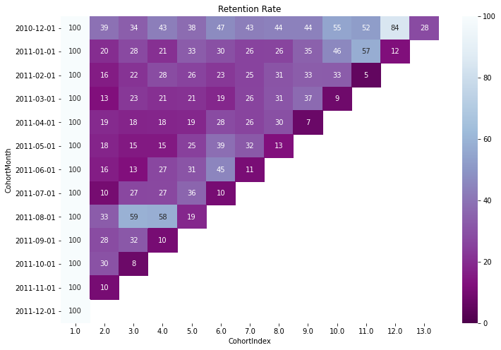
Retention Rate Table
cohort_counts = df.groupby(['CohortMonth', 'CohortIndex'])\
[['CustomerID']].count().unstack()
cohort_counts
| CustomerID | |||||||||||||
|---|---|---|---|---|---|---|---|---|---|---|---|---|---|
| CohortIndex | 1.0 | 2.0 | 3.0 | 4.0 | 5.0 | 6.0 | 7.0 | 8.0 | 9.0 | 10.0 | 11.0 | 12.0 | 13.0 |
| CohortMonth | |||||||||||||
| 2010-12-01 | 25670.0 | 10111.0 | 8689.0 | 11121.0 | 9628.0 | 11946.0 | 11069.0 | 11312.0 | 11316.0 | 14098.0 | 13399.0 | 21677.0 | 7173.0 |
| 2011-01-01 | 10877.0 | 2191.0 | 3012.0 | 2290.0 | 3603.0 | 3214.0 | 2776.0 | 2844.0 | 3768.0 | 4987.0 | 6248.0 | 1334.0 | NaN |
| 2011-02-01 | 8826.0 | 1388.0 | 1909.0 | 2487.0 | 2266.0 | 2012.0 | 2241.0 | 2720.0 | 2940.0 | 2916.0 | 451.0 | NaN | NaN |
| 2011-03-01 | 11349.0 | 1421.0 | 2598.0 | 2372.0 | 2435.0 | 2103.0 | 2942.0 | 3528.0 | 4214.0 | 967.0 | NaN | NaN | NaN |
| 2011-04-01 | 7185.0 | 1398.0 | 1284.0 | 1296.0 | 1343.0 | 2007.0 | 1869.0 | 2130.0 | 513.0 | NaN | NaN | NaN | NaN |
| 2011-05-01 | 6041.0 | 1075.0 | 906.0 | 917.0 | 1493.0 | 2329.0 | 1949.0 | 764.0 | NaN | NaN | NaN | NaN | NaN |
| 2011-06-01 | 5646.0 | 905.0 | 707.0 | 1511.0 | 1738.0 | 2545.0 | 616.0 | NaN | NaN | NaN | NaN | NaN | NaN |
| 2011-07-01 | 4938.0 | 501.0 | 1314.0 | 1336.0 | 1760.0 | 517.0 | NaN | NaN | NaN | NaN | NaN | NaN | NaN |
| 2011-08-01 | 4818.0 | 1591.0 | 2831.0 | 2801.0 | 899.0 | NaN | NaN | NaN | NaN | NaN | NaN | NaN | NaN |
| 2011-09-01 | 8225.0 | 2336.0 | 2608.0 | 862.0 | NaN | NaN | NaN | NaN | NaN | NaN | NaN | NaN | NaN |
| 2011-10-01 | 11500.0 | 3499.0 | 869.0 | NaN | NaN | NaN | NaN | NaN | NaN | NaN | NaN | NaN | NaN |
| 2011-11-01 | 10821.0 | 1100.0 | NaN | NaN | NaN | NaN | NaN | NaN | NaN | NaN | NaN | NaN | NaN |
| 2011-12-01 | 961.0 | NaN | NaN | NaN | NaN | NaN | NaN | NaN | NaN | NaN | NaN | NaN | NaN |
cohort_size = cohort_counts.iloc[:,0];
cohort_size
CohortMonth
2010-12-01    25670.0
2011-01-01    10877.0
2011-02-01     8826.0
2011-03-01    11349.0
2011-04-01     7185.0
2011-05-01     6041.0
2011-06-01     5646.0
2011-07-01     4938.0
2011-08-01     4818.0
2011-09-01     8225.0
2011-10-01    11500.0
2011-11-01    10821.0
2011-12-01      961.0
Name: (CustomerID, 1.0), dtype: float64
retention = (cohort_counts.divide(cohort_size, axis=0)*100).round(3)
retention.columns = retention.columns.droplevel()
retention.index = retention.index.astype('str')
fig, ax = plt.subplots(1,1, figsize=(12,8))
sns.heatmap(data=retention, annot=True, fmt='0.0f', ax =ax, vmin = 0.0,vmax = 100,cmap="BuPu_r")
ax.set_title('Retention Rate')
plt.show()
# loc, labels = plt.xticks(); labels
# labels[0]
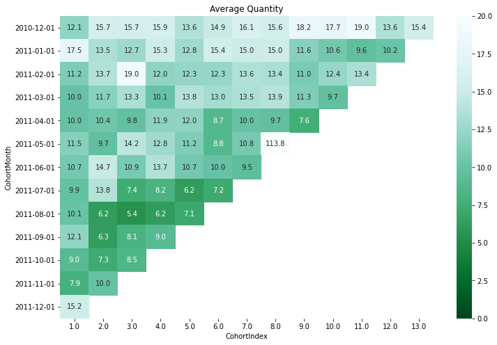
Average Quantity each cohort
cohort_counts = df.groupby(['CohortMonth', 'CohortIndex'])\
[['Quantity']].mean().unstack()
cohort_counts.round(1)
| Quantity | |||||||||||||
|---|---|---|---|---|---|---|---|---|---|---|---|---|---|
| CohortIndex | 1.0 | 2.0 | 3.0 | 4.0 | 5.0 | 6.0 | 7.0 | 8.0 | 9.0 | 10.0 | 11.0 | 12.0 | 13.0 |
| CohortMonth | |||||||||||||
| 2010-12-01 | 12.1 | 15.7 | 15.7 | 15.9 | 13.6 | 14.9 | 16.1 | 15.6 | 18.2 | 17.7 | 19.0 | 13.6 | 15.4 |
| 2011-01-01 | 17.5 | 13.5 | 12.7 | 15.3 | 12.8 | 15.4 | 15.0 | 15.0 | 11.6 | 10.6 | 9.6 | 10.2 | NaN |
| 2011-02-01 | 11.2 | 13.7 | 19.0 | 12.0 | 12.3 | 12.3 | 13.6 | 13.4 | 11.0 | 12.4 | 13.4 | NaN | NaN |
| 2011-03-01 | 10.0 | 11.7 | 13.3 | 10.1 | 13.8 | 13.0 | 13.5 | 13.9 | 11.3 | 9.7 | NaN | NaN | NaN |
| 2011-04-01 | 10.0 | 10.4 | 9.8 | 11.9 | 12.0 | 8.7 | 10.0 | 9.7 | 7.6 | NaN | NaN | NaN | NaN |
| 2011-05-01 | 11.5 | 9.7 | 14.2 | 12.8 | 11.2 | 8.8 | 10.8 | 113.8 | NaN | NaN | NaN | NaN | NaN |
| 2011-06-01 | 10.7 | 14.7 | 10.9 | 13.7 | 10.7 | 10.0 | 9.5 | NaN | NaN | NaN | NaN | NaN | NaN |
| 2011-07-01 | 9.9 | 13.8 | 7.4 | 8.2 | 6.2 | 7.2 | NaN | NaN | NaN | NaN | NaN | NaN | NaN |
| 2011-08-01 | 10.1 | 6.2 | 5.4 | 6.2 | 7.1 | NaN | NaN | NaN | NaN | NaN | NaN | NaN | NaN |
| 2011-09-01 | 12.1 | 6.3 | 8.1 | 9.0 | NaN | NaN | NaN | NaN | NaN | NaN | NaN | NaN | NaN |
| 2011-10-01 | 9.0 | 7.3 | 8.5 | NaN | NaN | NaN | NaN | NaN | NaN | NaN | NaN | NaN | NaN |
| 2011-11-01 | 7.9 | 10.0 | NaN | NaN | NaN | NaN | NaN | NaN | NaN | NaN | NaN | NaN | NaN |
| 2011-12-01 | 15.2 | NaN | NaN | NaN | NaN | NaN | NaN | NaN | NaN | NaN | NaN | NaN | NaN |
avg_quantity = cohort_counts.round(1)
avg_quantity.columns = avg_quantity.columns.droplevel()
avg_quantity.index = avg_quantity.index.astype('str')
fig, ax = plt.subplots(1,1, figsize=(12,8))
sns.heatmap(data=avg_quantity, annot=True, fmt='0.1f', ax =ax, vmin = 0.0, vmax = 20, cmap="BuGn_r")
ax.set_title('Average Quantity')
plt.show()
RFM Analysis
Concepts
Recency, Frequency and Monetary Value Calculations
Recency
When was last order?
Number of days since last purchase/ last visit/ last login
Frequency
Number of purchases in given period (3 - 6 or 12 months)
How many or how often customer used the product of company
Bigger Value => More engaged customer
Not VIP [ Need to associate to monetary value for that]
Monetary
Total amount of money spent in period selected above
Differentiate between MVP/ VIP

RFM values can be grouped in several ways :-
Percentiles eg quantiles
Pareto 80/20 Cut
Custom based on business Knowledge
For percentile implementation
Sort customers based on that metric
Break customers into a pre defined number of groups of equal size
Assign a label to each group
RFM Calculations
df['TotalSum'] = df['UnitPrice']*df['Quantity']
df.head()
| InvoiceNo | StockCode | Description | Quantity | InvoiceDate | UnitPrice | CustomerID | Country | InvoiceMonth | CohortMonth | CohortIndex | TotalSum | |
|---|---|---|---|---|---|---|---|---|---|---|---|---|
| 0 | 536365 | 85123A | WHITE HANGING HEART T-LIGHT HOLDER | 6 | 2010-12-01 08:26:00 | 2.55 | 17850.0 | United Kingdom | 2010-12-01 | 2010-12-01 | 1.0 | 15.30 |
| 1 | 536365 | 71053 | WHITE METAL LANTERN | 6 | 2010-12-01 08:26:00 | 3.39 | 17850.0 | United Kingdom | 2010-12-01 | 2010-12-01 | 1.0 | 20.34 |
| 2 | 536365 | 84406B | CREAM CUPID HEARTS COAT HANGER | 8 | 2010-12-01 08:26:00 | 2.75 | 17850.0 | United Kingdom | 2010-12-01 | 2010-12-01 | 1.0 | 22.00 |
| 3 | 536365 | 84029G | KNITTED UNION FLAG HOT WATER BOTTLE | 6 | 2010-12-01 08:26:00 | 3.39 | 17850.0 | United Kingdom | 2010-12-01 | 2010-12-01 | 1.0 | 20.34 |
| 4 | 536365 | 84029E | RED WOOLLY HOTTIE WHITE HEART. | 6 | 2010-12-01 08:26:00 | 3.39 | 17850.0 | United Kingdom | 2010-12-01 | 2010-12-01 | 1.0 | 20.34 |
df.InvoiceDate.dt.date.min(), df.InvoiceDate.dt.date.max()
(datetime.date(2010, 12, 1), datetime.date(2011, 12, 9))
In real world,
We would work with most recent snapshot of day from today or yesterday
snapshot_date = df['InvoiceDate'].max() + dt.timedelta(days=1)
snapshot_date
Timestamp('2011-12-10 12:50:00')
rfm = df.groupby(['CustomerID'])\
.agg({'InvoiceDate': lambda x : (snapshot_date - x.max()).days,
      'InvoiceNo': 'count',
      'TotalSum': 'sum'})

# rfm = df.groupby(['CustomerID'])\
# .agg({'Recency': lambda x : (snapshot_date - x.max()).days,
#       'Frequency': 'count',
#       'MonetaryValue': 'sum'})
rfm.rename(columns={'InvoiceDate':'Recency',
                    'InvoiceNo': 'Frequency',
                    'TotalSum': 'MonetaryValue'},
           inplace = True,
        )

rfm
| Recency | Frequency | MonetaryValue | |
|---|---|---|---|
| CustomerID | |||
| 12346.0 | 326.0 | 1 | 77183.60 |
| 12347.0 | 2.0 | 182 | 4310.00 |
| 12348.0 | 75.0 | 31 | 1797.24 |
| 12349.0 | 19.0 | 73 | 1757.55 |
| 12350.0 | 310.0 | 17 | 334.40 |
| ... | ... | ... | ... |
| 18280.0 | 278.0 | 10 | 180.60 |
| 18281.0 | 181.0 | 7 | 80.82 |
| 18282.0 | 8.0 | 12 | 178.05 |
| 18283.0 | 4.0 | 721 | 2045.53 |
| 18287.0 | 43.0 | 70 | 1837.28 |
4372 rows × 3 columns
Tip
Recency
Better rating to customer who have been active more recently
Frequency & Monetary Value
Different rating / higher label (than above)-we want to spend more money & visit more often
Now let’s see the magic happen
RFM Segments
list(range(4,0,-1)), list(range(1,5))
([4, 3, 2, 1], [1, 2, 3, 4])
r_labels = range(4, 0, -1)
f_labels = range(1,5)
m_labels = range(1,5)

r_labels, f_labels, m_labels
(range(4, 0, -1), range(1, 5), range(1, 5))
pd.qcut(list(range(1,101)), q=4, labels=r_labels)
[4, 4, 4, 4, 4, ..., 1, 1, 1, 1, 1]
Length: 100
Categories (4, int64): [4 < 3 < 2 < 1]
r_quartiles = pd.qcut(rfm['Recency'], q=4, labels=r_labels)
r_quartiles
CustomerID
12346.0    1
12347.0    4
12348.0    2
12349.0    3
12350.0    1
          ..
18280.0    1
18281.0    1
18282.0    4
18283.0    4
18287.0    3
Name: Recency, Length: 4372, dtype: category
Categories (4, int64): [4 < 3 < 2 < 1]
f_quartiles = pd.qcut(rfm['Frequency'], q=4, labels=f_labels)
f_quartiles
CustomerID
12346.0    1
12347.0    4
12348.0    2
12349.0    3
12350.0    1
          ..
18280.0    1
18281.0    1
18282.0    1
18283.0    4
18287.0    3
Name: Frequency, Length: 4372, dtype: category
Categories (4, int64): [1 < 2 < 3 < 4]
m_quartiles = pd.qcut(rfm['MonetaryValue'], q=4, labels=m_labels)
m_quartiles
CustomerID
12346.0    4
12347.0    4
12348.0    4
12349.0    4
12350.0    2
          ..
18280.0    1
18281.0    1
18282.0    1
18283.0    4
18287.0    4
Name: MonetaryValue, Length: 4372, dtype: category
Categories (4, int64): [1 < 2 < 3 < 4]
rfm = rfm.assign(R=r_quartiles, F=f_quartiles, M=m_quartiles)
rfm
| Recency | Frequency | MonetaryValue | R | F | M | |
|---|---|---|---|---|---|---|
| CustomerID | ||||||
| 12346.0 | 326.0 | 1 | 77183.60 | 1 | 1 | 4 |
| 12347.0 | 2.0 | 182 | 4310.00 | 4 | 4 | 4 |
| 12348.0 | 75.0 | 31 | 1797.24 | 2 | 2 | 4 |
| 12349.0 | 19.0 | 73 | 1757.55 | 3 | 3 | 4 |
| 12350.0 | 310.0 | 17 | 334.40 | 1 | 1 | 2 |
| ... | ... | ... | ... | ... | ... | ... |
| 18280.0 | 278.0 | 10 | 180.60 | 1 | 1 | 1 |
| 18281.0 | 181.0 | 7 | 80.82 | 1 | 1 | 1 |
| 18282.0 | 8.0 | 12 | 178.05 | 4 | 1 | 1 |
| 18283.0 | 4.0 | 721 | 2045.53 | 4 | 4 | 4 |
| 18287.0 | 43.0 | 70 | 1837.28 | 3 | 3 | 4 |
4372 rows × 6 columns
# rfm['RFMSegment'] = pd.to_numeric(rfm.R, downcast='integer').astype('str') +\
#                 pd.to_numeric(rfm.F, downcast='integer').astype('str')+\
#                 pd.to_numeric(rfm.M, downcast='integer').astype('str')


rfm.info()

# def str_val(x):
#     return str(int(x['R']))+str(x['F'])+str(x['M'])
# rfm['RFMSegment'] = rfm.apply(str_val, axis=1)
# rfm
<class 'pandas.core.frame.DataFrame'>
CategoricalIndex: 4372 entries, 12346.0 to 18287.0
Data columns (total 7 columns):
 #   Column         Non-Null Count  Dtype
---  ------         --------------  -----
 0   Recency        4338 non-null   float64
 1   Frequency      4372 non-null   int64
 2   MonetaryValue  4372 non-null   float64
 3   R              4338 non-null   category
 4   F              4372 non-null   category
 5   M              4372 non-null   category
 6   RFMSegment     4372 non-null   object
dtypes: category(3), float64(2), int64(1), object(1)
memory usage: 352.5+ KB
rfm[rfm.isnull()]
| Recency | Frequency | MonetaryValue | R | F | M | RFMSegment | |
|---|---|---|---|---|---|---|---|
| CustomerID | |||||||
| 12346.0 | NaN | NaN | NaN | NaN | NaN | NaN | NaN |
| 12347.0 | NaN | NaN | NaN | NaN | NaN | NaN | NaN |
| 12348.0 | NaN | NaN | NaN | NaN | NaN | NaN | NaN |
| 12349.0 | NaN | NaN | NaN | NaN | NaN | NaN | NaN |
| 12350.0 | NaN | NaN | NaN | NaN | NaN | NaN | NaN |
| ... | ... | ... | ... | ... | ... | ... | ... |
| 18280.0 | NaN | NaN | NaN | NaN | NaN | NaN | NaN |
| 18281.0 | NaN | NaN | NaN | NaN | NaN | NaN | NaN |
| 18282.0 | NaN | NaN | NaN | NaN | NaN | NaN | NaN |
| 18283.0 | NaN | NaN | NaN | NaN | NaN | NaN | NaN |
| 18287.0 | NaN | NaN | NaN | NaN | NaN | NaN | NaN |
4372 rows × 7 columns
rfm = rfm.dropna()
rfm.info()
<class 'pandas.core.frame.DataFrame'>
CategoricalIndex: 4338 entries, 12346.0 to 18287.0
Data columns (total 7 columns):
 #   Column         Non-Null Count  Dtype
---  ------         --------------  -----
 0   Recency        4338 non-null   float64
 1   Frequency      4338 non-null   int64
 2   MonetaryValue  4338 non-null   float64
 3   R              4338 non-null   category
 4   F              4338 non-null   category
 5   M              4338 non-null   category
 6   RFMSegment     4338 non-null   object
dtypes: category(3), float64(2), int64(1), object(1)
memory usage: 351.3+ KB
rfm['RFMSegment'] = pd.to_numeric(rfm.R, downcast='integer').astype('str') +\
                pd.to_numeric(rfm.F, downcast='integer').astype('str')+\
                pd.to_numeric(rfm.M, downcast='integer').astype('str')
rfm
| Recency | Frequency | MonetaryValue | R | F | M | RFMSegment | RFMScore | |
|---|---|---|---|---|---|---|---|---|
| CustomerID | ||||||||
| 12346.0 | 326.0 | 1 | 77183.60 | 1 | 1 | 4 | 114 | 6 |
| 12347.0 | 2.0 | 182 | 4310.00 | 4 | 4 | 4 | 444 | 12 |
| 12348.0 | 75.0 | 31 | 1797.24 | 2 | 2 | 4 | 224 | 8 |
| 12349.0 | 19.0 | 73 | 1757.55 | 3 | 3 | 4 | 334 | 10 |
| 12350.0 | 310.0 | 17 | 334.40 | 1 | 1 | 2 | 112 | 4 |
| ... | ... | ... | ... | ... | ... | ... | ... | ... |
| 18280.0 | 278.0 | 10 | 180.60 | 1 | 1 | 1 | 111 | 3 |
| 18281.0 | 181.0 | 7 | 80.82 | 1 | 1 | 1 | 111 | 3 |
| 18282.0 | 8.0 | 12 | 178.05 | 4 | 1 | 1 | 411 | 6 |
| 18283.0 | 4.0 | 721 | 2045.53 | 4 | 4 | 4 | 444 | 12 |
| 18287.0 | 43.0 | 70 | 1837.28 | 3 | 3 | 4 | 334 | 10 |
4338 rows × 8 columns
rfm['RFMScore'] = rfm[['R', 'F', 'M']].sum(axis=1)
rfm
| Recency | Frequency | MonetaryValue | R | F | M | RFMSegment | RFMScore | |
|---|---|---|---|---|---|---|---|---|
| CustomerID | ||||||||
| 12346.0 | 326.0 | 1 | 77183.60 | 1 | 1 | 4 | 114 | 6 |
| 12347.0 | 2.0 | 182 | 4310.00 | 4 | 4 | 4 | 444 | 12 |
| 12348.0 | 75.0 | 31 | 1797.24 | 2 | 2 | 4 | 224 | 8 |
| 12349.0 | 19.0 | 73 | 1757.55 | 3 | 3 | 4 | 334 | 10 |
| 12350.0 | 310.0 | 17 | 334.40 | 1 | 1 | 2 | 112 | 4 |
| ... | ... | ... | ... | ... | ... | ... | ... | ... |
| 18280.0 | 278.0 | 10 | 180.60 | 1 | 1 | 1 | 111 | 3 |
| 18281.0 | 181.0 | 7 | 80.82 | 1 | 1 | 1 | 111 | 3 |
| 18282.0 | 8.0 | 12 | 178.05 | 4 | 1 | 1 | 411 | 6 |
| 18283.0 | 4.0 | 721 | 2045.53 | 4 | 4 | 4 | 444 | 12 |
| 18287.0 | 43.0 | 70 | 1837.28 | 3 | 3 | 4 | 334 | 10 |
4338 rows × 8 columns
Analyzing Segments
rfm.groupby(['RFMSegment']).size().sort_values(ascending=False)
RFMSegment
444    451
111    374
344    217
122    202
211    175
      ...
124      7
314      7
414      6
142      3
441      3
Length: 61, dtype: int64
Filtering RFM Segments
rfm[rfm['RFMSegment'] =='111'].head()
| Recency | Frequency | MonetaryValue | R | F | M | RFMSegment | RFMScore | |
|---|---|---|---|---|---|---|---|---|
| CustomerID | ||||||||
| 12353.0 | 204.0 | 4 | 89.00 | 1 | 1 | 1 | 111 | 3 |
| 12361.0 | 287.0 | 10 | 189.90 | 1 | 1 | 1 | 111 | 3 |
| 12401.0 | 303.0 | 5 | 84.30 | 1 | 1 | 1 | 111 | 3 |
| 12402.0 | 323.0 | 11 | 225.60 | 1 | 1 | 1 | 111 | 3 |
| 12441.0 | 367.0 | 11 | 173.55 | 1 | 1 | 1 | 111 | 3 |
Summary Metrics RFMScore
rfm.groupby('RFMScore').agg({'Recency': 'mean',
                             'Frequency': 'mean',
                             'MonetaryValue':['mean','count']
                            }).round(1)
| Recency | Frequency | MonetaryValue | ||
|---|---|---|---|---|
| mean | mean | mean | count | |
| RFMScore | ||||
| 3 | 261.4 | 8.1 | 154.7 | 374 |
| 4 | 177.4 | 13.5 | 238.7 | 386 |
| 5 | 153.3 | 20.8 | 363.8 | 515 |
| 6 | 98.0 | 27.6 | 815.9 | 460 |
| 7 | 81.2 | 38.0 | 762.4 | 453 |
| 8 | 64.1 | 55.7 | 972.0 | 463 |
| 9 | 46.2 | 78.0 | 1787.7 | 415 |
| 10 | 32.5 | 109.9 | 2045.6 | 430 |
| 11 | 21.2 | 185.2 | 4034.2 | 391 |
| 12 | 7.2 | 368.0 | 9269.0 | 451 |
Segmentation based on RFM Score
def segments(x):
    if x['RFMScore'] > 9:
        return "GOLD"
    elif (x['RFMScore'] > 5) and (x['RFMScore'] <= 9):
        return "SILVER"
    else:
        return "BRONZE"

rfm['RFMSegment'] = rfm.apply(segments, axis=1)

rfm
| Recency | Frequency | MonetaryValue | R | F | M | RFMSegment | RFMScore | |
|---|---|---|---|---|---|---|---|---|
| CustomerID | ||||||||
| 12346.0 | 326.0 | 1 | 77183.60 | 1 | 1 | 4 | SILVER | 6 |
| 12347.0 | 2.0 | 182 | 4310.00 | 4 | 4 | 4 | GOLD | 12 |
| 12348.0 | 75.0 | 31 | 1797.24 | 2 | 2 | 4 | SILVER | 8 |
| 12349.0 | 19.0 | 73 | 1757.55 | 3 | 3 | 4 | GOLD | 10 |
| 12350.0 | 310.0 | 17 | 334.40 | 1 | 1 | 2 | BRONZE | 4 |
| ... | ... | ... | ... | ... | ... | ... | ... | ... |
| 18280.0 | 278.0 | 10 | 180.60 | 1 | 1 | 1 | BRONZE | 3 |
| 18281.0 | 181.0 | 7 | 80.82 | 1 | 1 | 1 | BRONZE | 3 |
| 18282.0 | 8.0 | 12 | 178.05 | 4 | 1 | 1 | SILVER | 6 |
| 18283.0 | 4.0 | 721 | 2045.53 | 4 | 4 | 4 | GOLD | 12 |
| 18287.0 | 43.0 | 70 | 1837.28 | 3 | 3 | 4 | GOLD | 10 |
4338 rows × 8 columns
rfm.groupby('RFMSegment').agg({'Recency': 'mean',
                             'Frequency': 'mean',
                             'MonetaryValue':['mean','count']
                            }).round(1)
| Recency | Frequency | MonetaryValue | ||
|---|---|---|---|---|
| mean | mean | mean | count | |
| RFMSegment | ||||
| BRONZE | 192.3 | 14.9 | 264.6 | 1275 |
| GOLD | 20.1 | 224.5 | 5218.0 | 1272 |
| SILVER | 73.0 | 49.2 | 1067.9 | 1791 |
Segmentation using KMeans
Attention
Symmetric distribution of variables(not skewed)
Variables with same average values
Variables with same variance
rfm[['Recency', 'Frequency', 'MonetaryValue']].describe()
| Recency | Frequency | MonetaryValue | |
|---|---|---|---|
| count | 4338.000000 | 4338.000000 | 4338.000000 |
| mean | 92.536422 | 90.523744 | 2048.688081 |
| std | 100.014169 | 225.506968 | 8985.230220 |
| min | 1.000000 | 1.000000 | 3.750000 |
| 25% | 18.000000 | 17.000000 | 306.482500 |
| 50% | 51.000000 | 41.000000 | 668.570000 |
| 75% | 142.000000 | 98.000000 | 1660.597500 |
| max | 374.000000 | 7676.000000 | 280206.020000 |
fig, axes = plt.subplots(ncols=1, nrows=3, figsize=(12,12))
(ax1, ax2, ax3) = axes

sns.distplot(rfm.Recency, label='Recency', ax= ax1)
sns.distplot(rfm.Frequency, label='Frequency', ax= ax2)
sns.distplot(rfm.MonetaryValue, label='MonetaryValue', ax= ax3)
plt.suptitle("RFM Distributions")
# plt.style.use('ggplot')
sns.set_theme()
sns.set_context("paper")
plt.tight_layout()
plt.show()
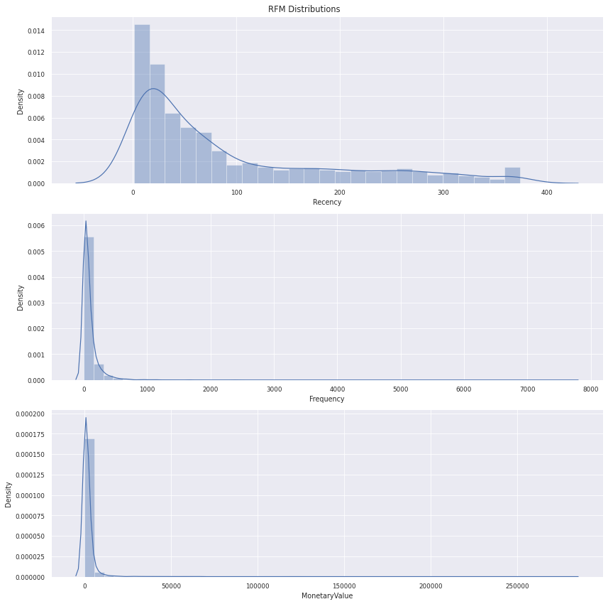
Review
From above table and figures
Mean of Recency & Frequency close ; Monetary Value vastly different
Variances are very different
Variable distribution is skewed
What should we do to fix it?
Transform and Scale the variables
Unskew the data using log transformation
Scale to same standard deviation
Store as a separate array to be used for clustering
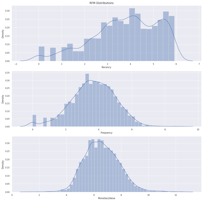
Fixing distributions
rfm_log = rfm[['Recency', 'Frequency', 'MonetaryValue']].apply(np.log, axis=1).round(3); rfm_log
| Recency | Frequency | MonetaryValue | |
|---|---|---|---|
| CustomerID | |||
| 12346.0 | 5.787 | 0.000 | 11.254 |
| 12347.0 | 0.693 | 5.204 | 8.369 |
| 12348.0 | 4.317 | 3.434 | 7.494 |
| 12349.0 | 2.944 | 4.290 | 7.472 |
| 12350.0 | 5.737 | 2.833 | 5.812 |
| ... | ... | ... | ... |
| 18280.0 | 5.628 | 2.303 | 5.196 |
| 18281.0 | 5.198 | 1.946 | 4.392 |
| 18282.0 | 2.079 | 2.485 | 5.182 |
| 18283.0 | 1.386 | 6.581 | 7.623 |
| 18287.0 | 3.761 | 4.248 | 7.516 |
4338 rows × 3 columns
fig, axes = plt.subplots(ncols=1, nrows=3, figsize=(12,12))
(ax1, ax2, ax3) = axes

sns.distplot(rfm_log.Recency, label='Recency', ax= ax1)
sns.distplot(rfm_log.Frequency, label='Frequency', ax= ax2)
sns.distplot(rfm_log.MonetaryValue, label='MonetaryValue', ax= ax3)
plt.suptitle("RFM Distributions")
# plt.style.use('ggplot')
sns.set_theme()
sns.set_context("paper")
plt.tight_layout()
plt.show()
log_transformer = FunctionTransformer(np.log)
rfm_log = log_transformer.fit_transform((rfm[['Recency', 'Frequency', 'MonetaryValue']])); rfm_log
| Recency | Frequency | MonetaryValue | |
|---|---|---|---|
| CustomerID | |||
| 12346.0 | 5.786897 | 0.000000 | 11.253942 |
| 12347.0 | 0.693147 | 5.204007 | 8.368693 |
| 12348.0 | 4.317488 | 3.433987 | 7.494007 |
| 12349.0 | 2.944439 | 4.290459 | 7.471676 |
| 12350.0 | 5.736572 | 2.833213 | 5.812338 |
| ... | ... | ... | ... |
| 18280.0 | 5.627621 | 2.302585 | 5.196285 |
| 18281.0 | 5.198497 | 1.945910 | 4.392224 |
| 18282.0 | 2.079442 | 2.484907 | 5.182064 |
| 18283.0 | 1.386294 | 6.580639 | 7.623412 |
| 18287.0 | 3.761200 | 4.248495 | 7.516041 |
4338 rows × 3 columns
sc = StandardScaler()
rfm_normalized = sc.fit_transform(rfm_log); rfm_normalized
array([[ 1.40989446, -2.77997755,  3.70020082],
       [-2.14649825,  1.16035591,  1.41325634],
       [ 0.38397128, -0.17985509,  0.7199513 ],
       ...,
       [-1.17860486, -0.89847328, -1.11257171],
       [-1.66255156,  2.20270486,  0.82252182],
       [-0.00442205,  0.43686843,  0.73741623]])
model = KMeans(n_clusters=3, max_iter=300, random_state=None)
model.fit_predict(rfm_normalized)
array([0, 2, 0, ..., 1, 2, 0], dtype=int32)
# pipeline = Pipeline([('lt', log_transformer), ('sc', sc), ('model', model)])
# pipeline.fit((rfm[['Recency', 'Frequency', 'MonetaryValue']]))
rfm['K_Cluster'] = model.fit_predict(rfm_normalized)
rfm
| Recency | Frequency | MonetaryValue | R | F | M | RFMSegment | RFMScore | K_Cluster | |
|---|---|---|---|---|---|---|---|---|---|
| CustomerID | |||||||||
| 12346.0 | 326.0 | 1 | 77183.60 | 1 | 1 | 4 | SILVER | 6 | 0 |
| 12347.0 | 2.0 | 182 | 4310.00 | 4 | 4 | 4 | GOLD | 12 | 1 |
| 12348.0 | 75.0 | 31 | 1797.24 | 2 | 2 | 4 | SILVER | 8 | 0 |
| 12349.0 | 19.0 | 73 | 1757.55 | 3 | 3 | 4 | GOLD | 10 | 0 |
| 12350.0 | 310.0 | 17 | 334.40 | 1 | 1 | 2 | BRONZE | 4 | 2 |
| ... | ... | ... | ... | ... | ... | ... | ... | ... | ... |
| 18280.0 | 278.0 | 10 | 180.60 | 1 | 1 | 1 | BRONZE | 3 | 2 |
| 18281.0 | 181.0 | 7 | 80.82 | 1 | 1 | 1 | BRONZE | 3 | 2 |
| 18282.0 | 8.0 | 12 | 178.05 | 4 | 1 | 1 | SILVER | 6 | 2 |
| 18283.0 | 4.0 | 721 | 2045.53 | 4 | 4 | 4 | GOLD | 12 | 1 |
| 18287.0 | 43.0 | 70 | 1837.28 | 3 | 3 | 4 | GOLD | 10 | 0 |
4338 rows × 9 columns
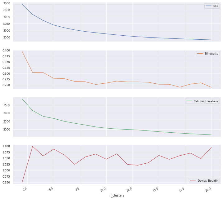
Determining Clusters
def score(n_clusters, X):
    km = KMeans(n_clusters=n_clusters, max_iter=300, random_state=None)
#     X = df[features]
    labels = km.fit_predict(X)
    SSE = km.inertia_
    Silhouette = metrics.silhouette_score(X, labels)
    CHS = metrics.calinski_harabasz_score(X, labels)
    DBS = metrics.davies_bouldin_score(X, labels)
    return {'SSE':SSE, 'Silhouette': Silhouette, 'Calinski_Harabasz': CHS, 'Davies_Bouldin':DBS, 'model':km}
rfm_normalized
array([[ 1.40989446, -2.77997755,  3.70020082],
       [-2.14649825,  1.16035591,  1.41325634],
       [ 0.38397128, -0.17985509,  0.7199513 ],
       ...,
       [-1.17860486, -0.89847328, -1.11257171],
       [-1.66255156,  2.20270486,  0.82252182],
       [-0.00442205,  0.43686843,  0.73741623]])
score(3,rfm_normalized)
{'SSE': 5314.652651827099,
 'Silhouette': 0.30360827075999475,
 'Calinski_Harabasz': 3140.104478514454,
 'Davies_Bouldin': 1.0979475974673056,
 'model': KMeans(n_clusters=3)}
df_cluster_scorer = pd.DataFrame()
df_cluster_scorer['n_clusters'] = list(range(2, 21))

df_cluster_scorer['SSE'],df_cluster_scorer['Silhouette'],\
df_cluster_scorer['Calinski_Harabasz'], df_cluster_scorer['Davies_Bouldin'],\
df_cluster_scorer['model'] = zip(*df_cluster_scorer['n_clusters'].map(lambda row: score(row, rfm_normalized).values()))

df_cluster_scorer
| n_clusters | SSE | Silhouette | Calinski_Harabasz | Davies_Bouldin | model | |
|---|---|---|---|---|---|---|
| 0 | 2 | 6883.800570 | 0.394879 | 3861.338471 | 0.949330 | KMeans(n_clusters=2) |
| 1 | 3 | 5314.671090 | 0.303543 | 3140.098839 | 1.098187 | KMeans(n_clusters=3) |
| 2 | 4 | 4440.249606 | 0.303142 | 2789.571405 | 1.058351 | KMeans(n_clusters=4) |
| 3 | 5 | 3766.516448 | 0.278121 | 2659.604851 | 1.086998 | KMeans(n_clusters=5) |
| 4 | 6 | 3367.186319 | 0.276715 | 2482.219740 | 1.063290 | KMeans(n_clusters=6) |
| 5 | 7 | 3047.059671 | 0.264630 | 2361.143844 | 1.023636 | KMeans(n_clusters=7) |
| 6 | 8 | 2802.571223 | 0.263357 | 2253.840597 | 1.054314 | KMeans() |
| 7 | 9 | 2628.342146 | 0.251287 | 2138.234736 | 1.066557 | KMeans(n_clusters=9) |
| 8 | 10 | 2462.012036 | 0.257576 | 2061.071283 | 1.045072 | KMeans(n_clusters=10) |
| 9 | 11 | 2306.640989 | 0.265960 | 2008.595889 | 1.067603 | KMeans(n_clusters=11) |
| 10 | 12 | 2156.386502 | 0.262470 | 1980.195815 | 1.023627 | KMeans(n_clusters=12) |
| 11 | 13 | 2030.706747 | 0.262547 | 1949.364270 | 1.019886 | KMeans(n_clusters=13) |
| 12 | 14 | 1941.866359 | 0.261126 | 1896.532025 | 1.030465 | KMeans(n_clusters=14) |
| 13 | 15 | 1866.874811 | 0.252259 | 1843.774752 | 1.060838 | KMeans(n_clusters=15) |
| 14 | 16 | 1796.873081 | 0.251948 | 1798.720522 | 1.044352 | KMeans(n_clusters=16) |
| 15 | 17 | 1736.265898 | 0.239702 | 1754.171350 | 1.059899 | KMeans(n_clusters=17) |
| 16 | 18 | 1681.586609 | 0.252776 | 1712.559874 | 1.070504 | KMeans(n_clusters=18) |
| 17 | 19 | 1621.520791 | 0.258585 | 1685.825098 | 1.047598 | KMeans(n_clusters=19) |
| 18 | 20 | 1576.767425 | 0.238955 | 1648.490285 | 1.094423 | KMeans(n_clusters=20) |
df_cluster_scorer.plot.line(subplots=True,x ='n_clusters', figsize=(12,12))
array([<AxesSubplot:xlabel='n_clusters'>,
       <AxesSubplot:xlabel='n_clusters'>,
       <AxesSubplot:xlabel='n_clusters'>,
       <AxesSubplot:xlabel='n_clusters'>], dtype=object)
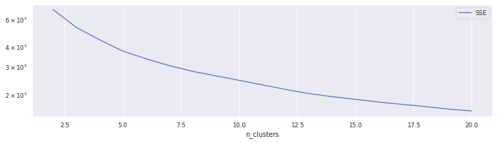
df_cluster_scorer.plot.line(y='SSE',x ='n_clusters',logy=True, figsize=(12,3))
<AxesSubplot:xlabel='n_clusters'>
pca = PCA(n_components=2, whiten=True)

# pca.fit_transform(rfm_normalized)

rfm['x'], rfm['y'] = zip(*(pca.fit_transform(rfm_normalized)))
rfm.head().T
| CustomerID | 12346.0 | 12347.0 | 12348.0 | 12349.0 | 12350.0 |
|---|---|---|---|---|---|
| Recency | 326 | 2 | 75 | 19 | 310 |
| Frequency | 1 | 182 | 31 | 73 | 17 |
| MonetaryValue | 77183.6 | 4310 | 1797.24 | 1757.55 | 334.4 |
| R | 1 | 4 | 2 | 3 | 1 |
| F | 1 | 4 | 2 | 3 | 1 |
| M | 4 | 4 | 4 | 4 | 2 |
| RFMSegment | SILVER | GOLD | SILVER | GOLD | BRONZE |
| RFMScore | 6 | 12 | 8 | 10 | 4 |
| K_Cluster | 0 | 1 | 0 | 0 | 2 |
| x | -0.107924 | 1.80756 | 0.0907543 | 0.683463 | -0.991831 |
| y | -2.03436 | 1.19585 | -0.684388 | 0.0950318 | -0.953282 |
rfm.groupby('K_Cluster').agg({'Recency': 'mean',
                             'Frequency': 'mean',
                             'MonetaryValue':['mean','count']
                            }).round(1)
| Recency | Frequency | MonetaryValue | ||
|---|---|---|---|---|
| mean | mean | mean | count | |
| K_Cluster | ||||
| 0 | 69.1 | 65.2 | 1164.3 | 1855 |
| 1 | 13.2 | 259.1 | 6536.1 | 961 |
| 2 | 171.3 | 14.9 | 293.2 | 1522 |
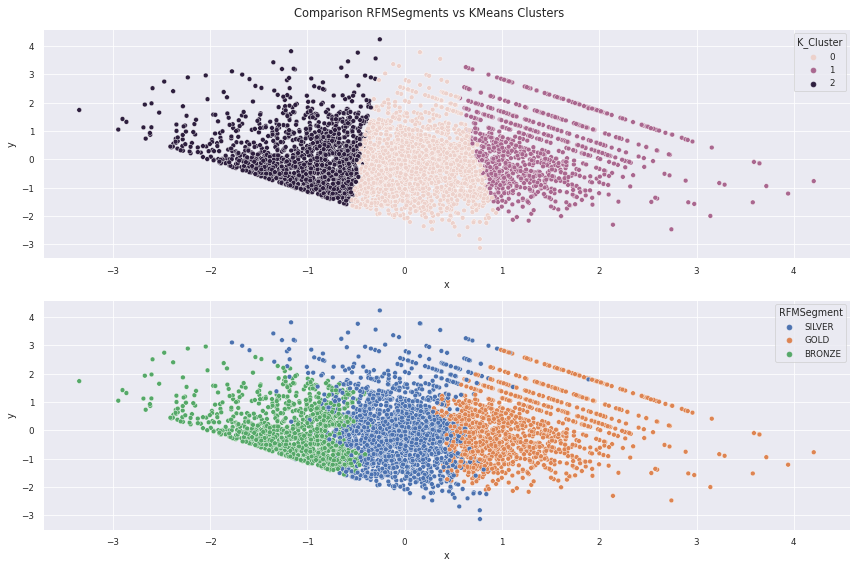
Visualization
# plt.scatter(rfm['x'], rfm['y'], c=rfm['K_Cluster'])
# # plt.scatter(rfm['x'], rfm['y'], c=rfm['RFMSegment'])
# # plt.show()
# plt.legend()
# plt.show()
fig, (ax1, ax2) = plt.subplots(nrows=2, ncols=1, figsize=(12, 8))
sns.scatterplot(data=rfm, x="x", y="y", hue='K_Cluster', ax=ax1)
sns.scatterplot(data=rfm, x="x", y="y", hue='RFMSegment', ax=ax2)
plt.suptitle("Comparison RFMSegments vs KMeans Clusters")
plt.tight_layout()
plt.show()
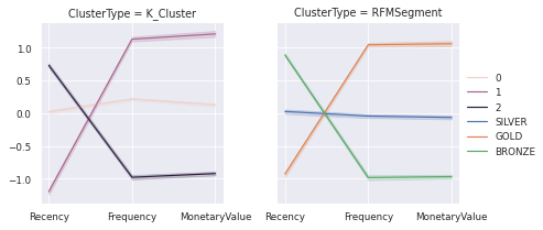
Comparing and Understanding Different Segments
Snake Plot
Market research technique to compare different segment
Visual representation of each segment’s attributes
Need data normalization (centering and scaling)
Plot each cluster’s average normalized value of each attribute
rfm
| Recency | Frequency | MonetaryValue | R | F | M | RFMSegment | RFMScore | K_Cluster | x | y | |
|---|---|---|---|---|---|---|---|---|---|---|---|
| CustomerID | |||||||||||
| 12346.0 | 326.0 | 1 | 77183.60 | 1 | 1 | 4 | SILVER | 6 | 0 | -0.107924 | -2.034364 |
| 12347.0 | 2.0 | 182 | 4310.00 | 4 | 4 | 4 | GOLD | 12 | 1 | 1.807565 | 1.195854 |
| 12348.0 | 75.0 | 31 | 1797.24 | 2 | 2 | 4 | SILVER | 8 | 0 | 0.090754 | -0.684388 |
| 12349.0 | 19.0 | 73 | 1757.55 | 3 | 3 | 4 | GOLD | 10 | 0 | 0.683463 | 0.095032 |
| 12350.0 | 310.0 | 17 | 334.40 | 1 | 1 | 2 | BRONZE | 4 | 2 | -0.991831 | -0.953282 |
| ... | ... | ... | ... | ... | ... | ... | ... | ... | ... | ... | ... |
| 18280.0 | 278.0 | 10 | 180.60 | 1 | 1 | 1 | BRONZE | 3 | 2 | -1.334170 | -0.453675 |
| 18281.0 | 181.0 | 7 | 80.82 | 1 | 1 | 1 | BRONZE | 3 | 2 | -1.606353 | 0.304837 |
| 18282.0 | 8.0 | 12 | 178.05 | 4 | 1 | 1 | SILVER | 6 | 2 | -0.425600 | 2.252207 |
| 18283.0 | 4.0 | 721 | 2045.53 | 4 | 4 | 4 | GOLD | 12 | 1 | 1.827859 | 0.453958 |
| 18287.0 | 43.0 | 70 | 1837.28 | 3 | 3 | 4 | GOLD | 10 | 0 | 0.487800 | -0.543167 |
4338 rows × 11 columns
rfm_normalized.shape
(4338, 3)
df_rfm_normalized = pd.DataFrame(rfm_normalized, index=rfm.index, columns =[['Recency', 'Frequency', 'MonetaryValue']])
df_rfm_normalized['K_Cluster'] = rfm['K_Cluster']
df_rfm_normalized['RFMSegment'] = rfm['RFMSegment']
df_rfm_normalized.reset_index(inplace=True)
df_rfm_normalized
| CustomerID | Recency | Frequency | MonetaryValue | K_Cluster | RFMSegment | |
|---|---|---|---|---|---|---|
| 0 | 12346.0 | 1.409894 | -2.779978 | 3.700201 | 0 | SILVER |
| 1 | 12347.0 | -2.146498 | 1.160356 | 1.413256 | 1 | GOLD |
| 2 | 12348.0 | 0.383971 | -0.179855 | 0.719951 | 0 | SILVER |
| 3 | 12349.0 | -0.574674 | 0.468643 | 0.702251 | 0 | GOLD |
| 4 | 12350.0 | 1.374758 | -0.634745 | -0.612996 | 2 | BRONZE |
| ... | ... | ... | ... | ... | ... | ... |
| 4333 | 18280.0 | 1.298690 | -1.036522 | -1.101300 | 2 | BRONZE |
| 4334 | 18281.0 | 0.999081 | -1.306587 | -1.738625 | 2 | BRONZE |
| 4335 | 18282.0 | -1.178605 | -0.898473 | -1.112572 | 2 | SILVER |
| 4336 | 18283.0 | -1.662552 | 2.202705 | 0.822522 | 1 | GOLD |
| 4337 | 18287.0 | -0.004422 | 0.436868 | 0.737416 | 0 | GOLD |
4338 rows × 6 columns
df_rfm_normalized.columns= [a[0] for a in df_rfm_normalized.columns.tolist()]
df_rfm_normalized.columns
Index(['CustomerID', 'Recency', 'Frequency', 'MonetaryValue', 'K_Cluster',
       'RFMSegment'],
      dtype='object')
df_rfm_melt = pd.melt(df_rfm_normalized,
                      id_vars=['CustomerID', 'K_Cluster', 'RFMSegment'],
                      value_vars=['Recency', 'Frequency', 'MonetaryValue'],
                      value_name = 'Value',
                      var_name = 'Metric'
                     )

df_rfm_melt
| CustomerID | K_Cluster | RFMSegment | Metric | Value | |
|---|---|---|---|---|---|
| 0 | 12346.0 | 0 | SILVER | Recency | 1.409894 |
| 1 | 12347.0 | 1 | GOLD | Recency | -2.146498 |
| 2 | 12348.0 | 0 | SILVER | Recency | 0.383971 |
| 3 | 12349.0 | 0 | GOLD | Recency | -0.574674 |
| 4 | 12350.0 | 2 | BRONZE | Recency | 1.374758 |
| ... | ... | ... | ... | ... | ... |
| 13009 | 18280.0 | 2 | BRONZE | MonetaryValue | -1.101300 |
| 13010 | 18281.0 | 2 | BRONZE | MonetaryValue | -1.738625 |
| 13011 | 18282.0 | 2 | SILVER | MonetaryValue | -1.112572 |
| 13012 | 18283.0 | 1 | GOLD | MonetaryValue | 0.822522 |
| 13013 | 18287.0 | 0 | GOLD | MonetaryValue | 0.737416 |
13014 rows × 5 columns
df_rfm_melt2 = pd.melt(df_rfm_melt,
                      id_vars=['CustomerID', 'Metric', 'Value'],
                      value_vars=['K_Cluster', 'RFMSegment'],
                      value_name='ClusterName',
                      var_name='ClusterType')
df_rfm_melt2
| CustomerID | Metric | Value | ClusterType | ClusterName | |
|---|---|---|---|---|---|
| 0 | 12346.0 | Recency | 1.409894 | K_Cluster | 0 |
| 1 | 12347.0 | Recency | -2.146498 | K_Cluster | 1 |
| 2 | 12348.0 | Recency | 0.383971 | K_Cluster | 0 |
| 3 | 12349.0 | Recency | -0.574674 | K_Cluster | 0 |
| 4 | 12350.0 | Recency | 1.374758 | K_Cluster | 2 |
| ... | ... | ... | ... | ... | ... |
| 26023 | 18280.0 | MonetaryValue | -1.101300 | RFMSegment | BRONZE |
| 26024 | 18281.0 | MonetaryValue | -1.738625 | RFMSegment | BRONZE |
| 26025 | 18282.0 | MonetaryValue | -1.112572 | RFMSegment | SILVER |
| 26026 | 18283.0 | MonetaryValue | 0.822522 | RFMSegment | GOLD |
| 26027 | 18287.0 | MonetaryValue | 0.737416 | RFMSegment | GOLD |
26028 rows × 5 columns
g = sns.FacetGrid(df_rfm_melt2, col='ClusterType')
g.map_dataframe(sns.lineplot, x="Metric", y="Value", hue='ClusterName', legend='brief')
g.add_legend()
<seaborn.axisgrid.FacetGrid at 0x7fca01f24640>
Relative Importance of segment attributes
Identify relative importance of each segment attribute
Calculate avg values of each clust
Calculate avg values of population
Calculate importance score by dividing them and subtracting 1 (ensures 0 is returned when cluster average equals population average)
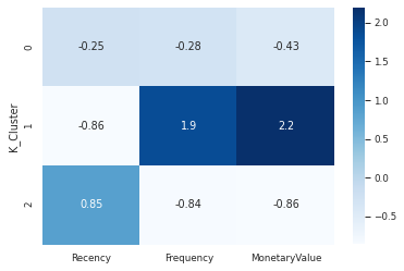
cluster_avg = rfm.groupby('K_Cluster').mean();
cluster_avg
| Recency | Frequency | MonetaryValue | RFMScore | x | y | |
|---|---|---|---|---|---|---|
| K_Cluster | ||||||
| 0 | 69.052291 | 65.239353 | 1164.318217 | 8.095957 | 0.135688 | -0.182712 |
| 1 | 13.169615 | 259.093652 | 6536.055567 | 11.264308 | 1.384201 | 0.246466 |
| 2 | 171.271353 | 14.904074 | 293.199212 | 4.455322 | -1.039368 | 0.067068 |
population_avg= rfm.mean()
population_avg
Recency          9.253642e+01
Frequency        9.052374e+01
MonetaryValue    2.048688e+03
RFMScore         7.520516e+00
K_Cluster        9.232365e-01
x                2.293130e-17
y                1.965540e-17
dtype: float64
cluster_avg = rfm.groupby('K_Cluster').mean();
population_avg= rfm.mean()
relative_imp = cluster_avg/population_avg -1
relative_imp = relative_imp[['Recency', 'Frequency', 'MonetaryValue']].round(2)
relative_imp
| Recency | Frequency | MonetaryValue | |
|---|---|---|---|
| K_Cluster | |||
| 0 | -0.25 | -0.28 | -0.43 |
| 1 | -0.86 | 1.86 | 2.19 |
| 2 | 0.85 | -0.84 | -0.86 |
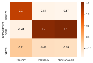
cluster_avg = rfm.groupby('RFMSegment').mean()
population_avg= rfm.mean()
prop_rfm = cluster_avg/population_avg -1
prop_rfm
| Recency | Frequency | MonetaryValue | RFMScore | K_Cluster | x | y | |
|---|---|---|---|---|---|---|---|
| RFMSegment | |||||||
| BRONZE | 1.078088 | -0.835441 | -0.870851 | -0.453417 | 1.128913 | -4.864229e+16 | -4.335882e+15 |
| GOLD | -0.783147 | 1.480533 | 1.546985 | 0.464861 | -0.204671 | 5.205352e+16 | 2.880894e+15 |
| SILVER | -0.211278 | -0.456756 | -0.478744 | -0.007368 | -0.658304 | -2.341240e+15 | 1.040621e+15 |
cluster_avg = rfm.groupby('RFMSegment').mean();
population_avg= rfm.mean()
prop_rfm = cluster_avg/population_avg -1
prop_rfm  = prop_rfm[['Recency', 'Frequency', 'MonetaryValue']].round(2)
prop_rfm
| Recency | Frequency | MonetaryValue | |
|---|---|---|---|
| RFMSegment | |||
| BRONZE | 1.08 | -0.84 | -0.87 |
| GOLD | -0.78 | 1.48 | 1.55 |
| SILVER | -0.21 | -0.46 | -0.48 |
sns.heatmap(data=relative_imp, annot=True, cmap='Blues')
<AxesSubplot:ylabel='K_Cluster'>
sns.heatmap(data=prop_rfm, annot=True, cmap='Oranges')
<AxesSubplot:ylabel='RFMSegment'>
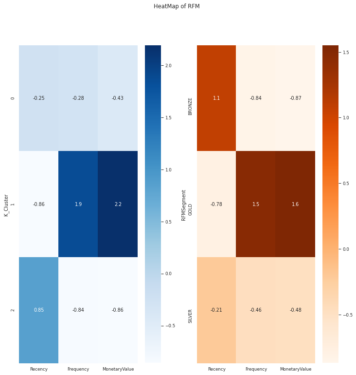
fig, (ax1, ax2) = plt.subplots(nrows=1, ncols=2,figsize=(12,12) )
sns.heatmap(data=relative_imp, annot=True, cmap='Blues', ax=ax1)
sns.heatmap(data=prop_rfm, annot=True, cmap='Oranges',ax =ax2)
plt.suptitle("HeatMap of RFM")
plt.show()
Pending
Tenure in RFM : Time since first transaction(How long customer has been with the company)